ALLPCB


Introduction
One common challenge in designs for smartwatches and fitness wearables is improving signal quality to obtain more accurate oxygen saturation (SpO2) measurements. Building on prior experience with spread-spectrum methods, the same techniques can be adapted to improve signal-to-noise ratio (SNR) in multi-sensor environments such as pulse oximetry.
Pulse Oximetry Example
The demonstration application used here is a reflective pulse oximeter. The block diagram is shown in Figure 1 and will be referenced throughout this article.
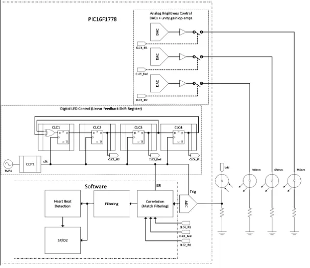
Figure 1. Reflective pulse oximeter (RPO) application block diagram.
In a typical clinical measurement, a finger clip uses red and infrared LEDs to measure heart rate and blood oxygen saturation. Advanced monitors in surgical settings may use up to eight wavelengths to measure heart rate, SpO2, carbon monoxide poisoning, and other parameters under general anesthesia.
When a sensor uses multiple signal sources (LEDs in pulse oximetry), there is a resource-sharing problem similar to that in multi-user communication systems. Each LED must share the same detector, typically a photodiode. The conventional approach is to activate each light source sequentially and take each measurement in turn. Each source therefore has its own time slot and the detector measures during that slot. This is time-division multiplexing (TDM).
The main drawback of TDM is that adding more sources requires more time to obtain measurements from each source, reducing the effective sampling rate per source. Since the measured signal (the arterial pulse) is time-varying, measurements can be biased by the acquisition order. A higher sampling rate mitigates these problems, but current practice also requires subtracting a background measurement from the source measurement.
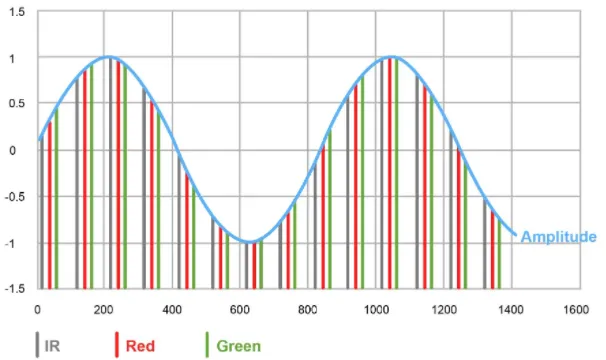
Figure 2. Sampling bias illustration.
Code-Division and Phase-Division Multiplexing
Many wireless systems use code-division multiple access (CDMA). In that approach, the system uses coding sequences with low cross-correlation so multiple users can coexist with limited crosstalk. In digital systems, the residual crosstalk can be negligible, but in precise analog measurements it can cause issues.
The technique used here for the pulse oximeter leverages maximal length (ML) sequences, which are also used to generate Gold codes. Instead of using multiple distinct sequences, we use a single ML sequence and apply phase shifts for each signal source. We call this phase-division multiplexing (PDM). PDM works because of specific properties of ML sequences.
Properties of Maximal Length (ML) Sequences
ML sequences are named because they cycle through the maximum number of non-zero states representable by a given number of bits. For n bits, the sequence repeats every 2^n - 1 chips. The output of an ML sequence contains nearly equal numbers of logical 1 and 0. It is common to map the sequence to values +1 and -1. With this representation, the autocorrelation of an ML sequence is impulse-like: a single peak of value 2^n - 1 at zero shift and flat -1 for all other shifts. If the output is zero-mean, the peak becomes 2^n - 1 and the off-peak correlations are zero. This means that repeating and shifting the same sequence allows signals to be separated by correlation. Figure 3 illustrates this behavior. The top plot shows the ML sequence; shifted versions generate the "red" and "IR" signals. The ADC sees the combined signal, and the bottom plot shows the circular cross-correlation between the reference and the measured signal. The two peaks correspond to the red and IR phase shifts, and all other shifts have zero correlation. This implies that up to 13 additional sensor sources can be injected without affecting the measurement period or other sources, which is a significant gain over conventional TDM.
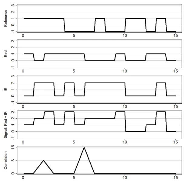
Figure 3. PDM example; axes are arbitrary units of time and amplitude.
Generating ML Sequences
ML sequences are generated using linear feedback shift registers (LFSRs), which can be implemented in hardware or software. LFSRs use a shift register of arbitrary length with taps whose outputs are XORed and fed back into the register input. Figure 4 shows an example LFSR. Table 1 lists effective LFSR parameters. The LFSR shown has n = 4 and tap = 3. The same LFSR configuration used in the demonstration was constructed with configurable logic cells.
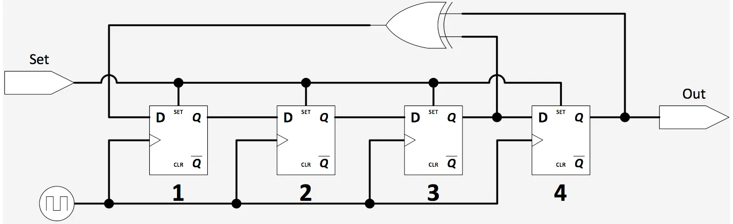
Figure 4. Linear feedback shift register (LFSR), size = 4, taps = 3.
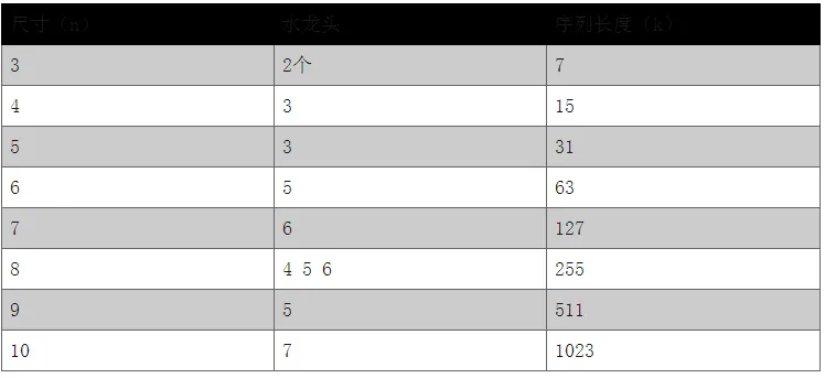
Table 1. LFSR tap parameters.
Correlation
The final step is correlation, implemented by multiplying the detector result with the LED state (+1 for on, -1 for off) and integrating or accumulating the product. In other words, when a source is on we add the detector result; when it is off we subtract it. This process can be performed in analog or digital form. In the application discussed here, ADC results were correlated. ADC conversions were triggered on the falling edge of the LFSR clock, and each conversion result was correlated in an interrupt.
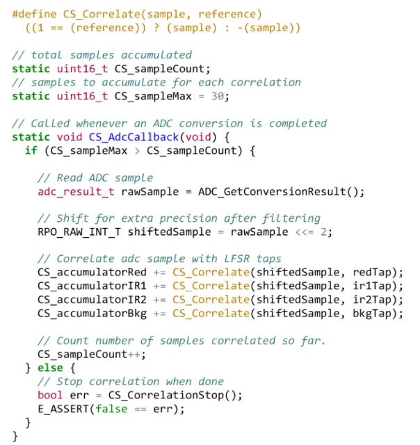
Figure 5. Correlation code example called on each ADC interrupt.
Results
Figures 6 and 7 show demonstration results for the pulse oximeter using the new PDM method and the older TDM method respectively. The plots show the correlated PDM result and the TDM result, resampled to match the correlation period. Each PDM sample represents 30 ADC samples. Each TDM sample represents 28 total samples ((3 sensors + 1 background) × 7). The PDM result exhibits a peak-to-peak amplitude roughly twice that of the TDM result. With PDM, each source has an effective 16 samples compared with seven samples per source in the TDM example. Adding additional light sources with PDM does not reduce the effective sample count per source (an LFSR of size 4 supports up to 15 sources), while with TDM each additional source consumes more time and reduces per-source sampling.
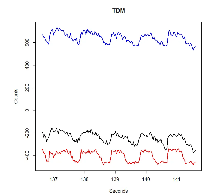
Figure 6. TDM correlation results: red 650 nm, blue 650 nm, black 940 nm.
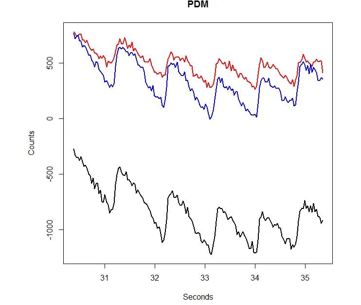
Figure 7. PDM correlation results: red 650 nm, blue 650 nm, black 940 nm.
Analysis
Because the only difference between the methods is the multiplexing scheme (TDM vs PDM), error propagation analysis can be applied to quantify trade-offs. Which method is better? If PDM is chosen, is it preferable to use a longer sequence or to repeat a shorter sequence for the same total time?
Assume the sum of sensor measurements is represented as:
For an ML sequence of length K = 2^n - 1, and mapping bits to +1 and -1, the correlation result is scaled by the number of chips where the source is active. For a length-15 ML sequence, the LED is on for 8 chips and off for 7 chips, so the source amplitude appears eight times while ambient contributes once. A general expression and error propagation are shown below.
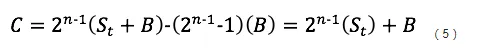
C = correlation result
St = sum of amplitudes from all signal sources
B = background
n = LFSR length
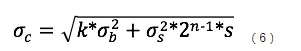
σ_c^2 = variance of correlated sample
σ_b = variance of background measurement
σ_s = variance of summed source measurements
K = 2^n - 1 = ML sequence length
S = number of sources
For TDM, the analysis is simpler when each source measurement equals S and the background equals B. Repeating the measurement m times scales the variance accordingly. These equations were placed in a spreadsheet to estimate when TDM or PDM is more suitable. On paper, TDM can outperform PDM when there are only one or two sources (for example, one red LED and one IR LED). For three or more sources, PDM is generally better (for example, red, IR, and green LEDs common in many heart-rate wearable devices).
Conclusions
Phase-division multiplexing can be applied to many sensor applications such as pulse oximetry and touch sensing. This article demonstrated how to generate multiplexed signals in hardware, how to correlate the multiplexed detector output to recover individual source signals, and provided statistical tools to compare PDM and TDM so designers can select the appropriate method for their application.