7 Hyperparameter Search Methods for Machine Learning

Introduction

Hyperparameter search is an essential step in the machine learning lifecycle, particularly for model performance. Correct hyperparameter selection can significantly improve model accuracy, generalization to unseen data, and convergence speed. Poor choices may lead to overfitting or underfitting.

Common hyperparameter examples include the learning rate in gradient-based algorithms or the tree depth in decision tree algorithms, which directly affect a model's ability to fit training data. Hyperparameter tuning involves searching a complex, high-dimensional space for the best configuration. The challenge lies not only in computational cost but also in balancing model complexity, generalization, and overfitting.

Method 1: Grid Search

Grid Search is a popular hyperparameter optimization method that systematically enumerates combinations of hyperparameters. It is simple and intuitive but can become very time-consuming and computationally intensive in high-dimensional parameter spaces.

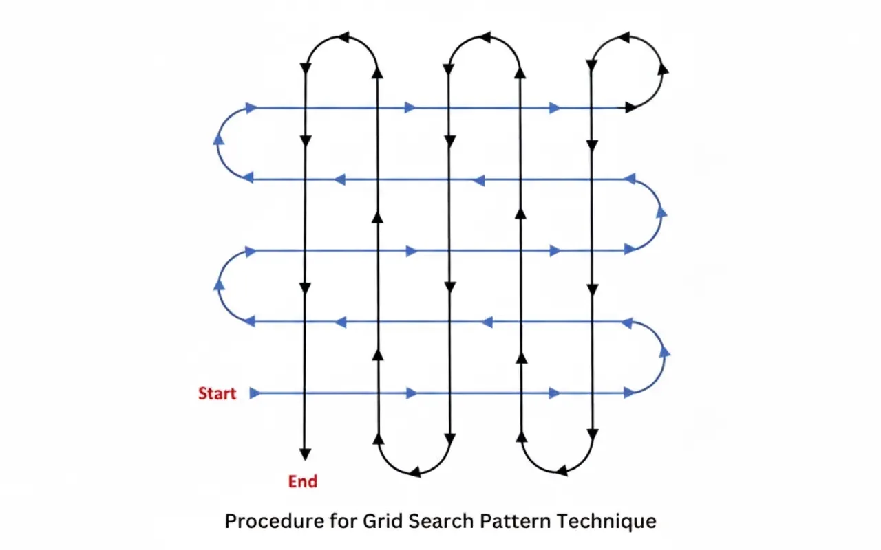
Grid Search generates all possible parameter combinations. For example, with two hyperparameters each taking three values, grid search will produce 9 different parameter combinations.

• Simple and interpretable: The concept is straightforward and easy to implement.
• Exhaustive (within the grid): If the grid is sufficiently dense, grid search can find the global optimum within that grid.
• Computationally expensive: The number of combinations grows exponentially with the number of parameters and values, which can lead to very high computational cost.

from sklearn import svm, datasetsfrom sklearn.model_selection import GridSearchCViris = datasets.load_iris()parameters = {'kernel': ('linear', 'rbf'), 'C': [1, 10]}svc = svm.SVC()clf = GridSearchCV(svc, parameters)clf.fit(iris.data, iris.target)sorted(clf.cv_results_.keys())

Method 2: Random Search

Random Search is another common hyperparameter optimization technique. Unlike grid search, it does not attempt to evaluate every possible parameter combination; instead, it samples parameter combinations randomly from the parameter space.

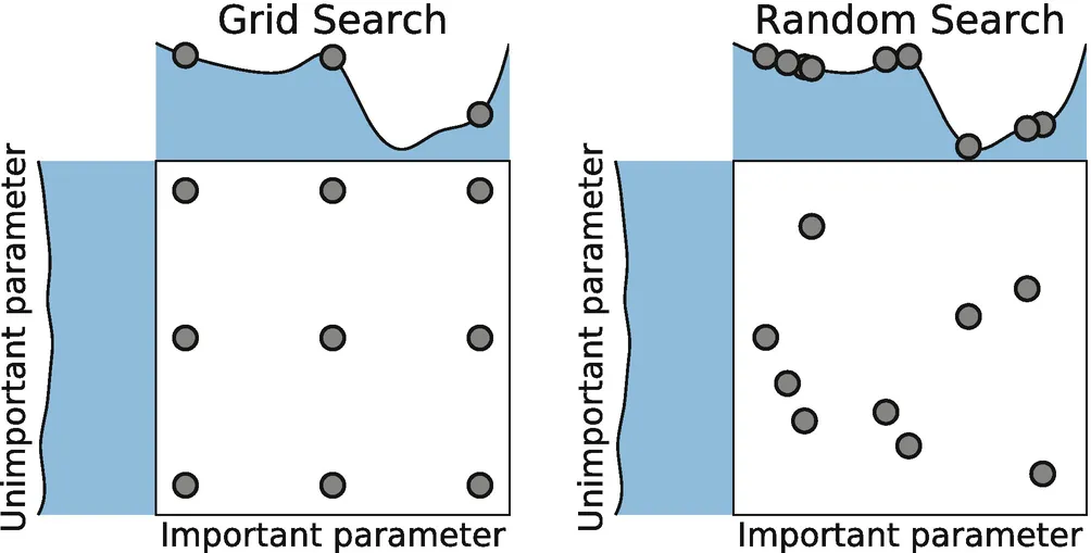
Random Search samples parameter values independently from specified distributions to form parameter combinations. Each draw is independent, so the same parameter value can appear in different combinations.

• Flexible: Random search can handle both continuous and discrete parameters easily.
• Avoids some local optima: Due to randomness, it is less likely to get stuck in local optima and has a better chance of finding the global optimum.
• Non-deterministic results: Different runs may yield different results because parameter combinations are chosen randomly.

from sklearn.datasets import load_irisfrom sklearn.linear_model import LogisticRegressionfrom sklearn.model_selection import RandomizedSearchCVfrom scipy.stats import uniformiris = load_iris()logistic = LogisticRegression(solver='saga', tol=1e-2, max_iter=200, random_state=0)distributions = dict(C=uniform(loc=0, scale=4), penalty=['l2', 'l1'])clf = RandomizedSearchCV(logistic, distributions, random_state=0)search = clf.fit(iris.data, iris.target)search.best_params_

Method 3: Bayesian Optimization

Bayesian optimization builds a probabilistic model that predicts the objective function's behavior, typically model performance metrics such as accuracy or loss, across different hyperparameter combinations.

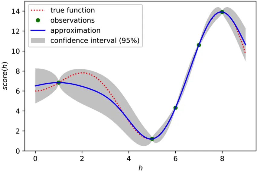
The probabilistic model is often based on a Gaussian process, which uses observed data points—previously evaluated hyperparameter combinations and their performance—to predict the performance of new combinations and select promising candidates for evaluation.

• Balances exploration and exploitation: Bayesian optimization mitigates issues like sparse gradients and the exploration-exploitation trade-off found in traditional methods.
• Improved efficiency: It can more efficiently search high-dimensional parameter spaces and reduce the number of evaluations needed.

def black_box_function(x, y):    """Function with unknown internals we wish to maximize."""    return -x**2 - (y - 1)**2 + 1from bayes_opt import BayesianOptimizationpbounds = {'x': (2, 4), 'y': (-3, 3)}optimizer = BayesianOptimization(    f=black_box_function,    pbounds=pbounds,    random_state=1,)optimizer.maximize(    init_points=2,    n_iter=3,)

Method 4: Simulated Annealing

Simulated Annealing (SA) is a probabilistic heuristic search algorithm inspired by the annealing process in physics. It mimics molecular motion during metal annealing to solve complex optimization problems.

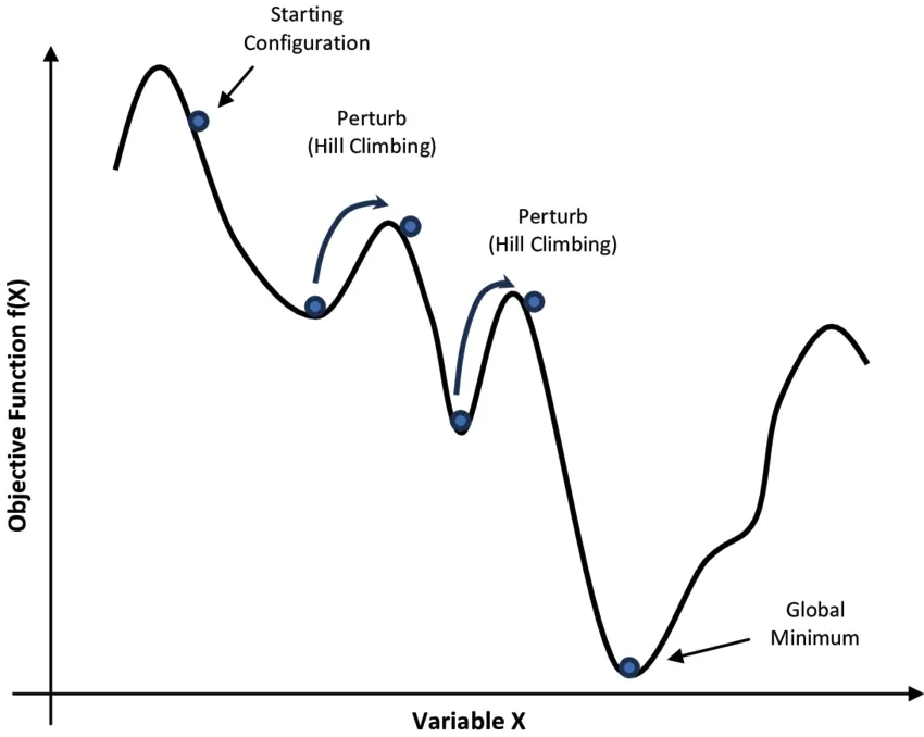
The algorithm starts from an initial solution with a high initial temperature. A new solution is randomly generated in the current solution's neighborhood and its objective value is computed. If the new solution is better, it is accepted; if worse, it may still be accepted with a certain probability.

• Global search capability: Simulated annealing can explore the entire solution space and is useful for problems with many local optima.
• Stochasticity: Random perturbations and occasional acceptance of worse solutions increase the chance of escaping local optima.

Method 5: Genetic Algorithm

Genetic Algorithms (GA) are optimization methods inspired by natural evolution. They apply mechanisms like selection, crossover, and mutation to a population of candidate solutions.

An initial population is generated randomly, with each individual encoded as a chromosome. Crossover combines parts of two individuals to produce offspring, and random mutations introduce genetic variation.

• Global search capability: Population-based search helps explore the search space and avoid local optima.
• Parallelism: GA is naturally amenable to parallel computation since evaluations of individuals are largely independent.

Method 6: Successive Halving

Successive Halving is an efficient hyperparameter optimization method particularly suited for large-scale searches.

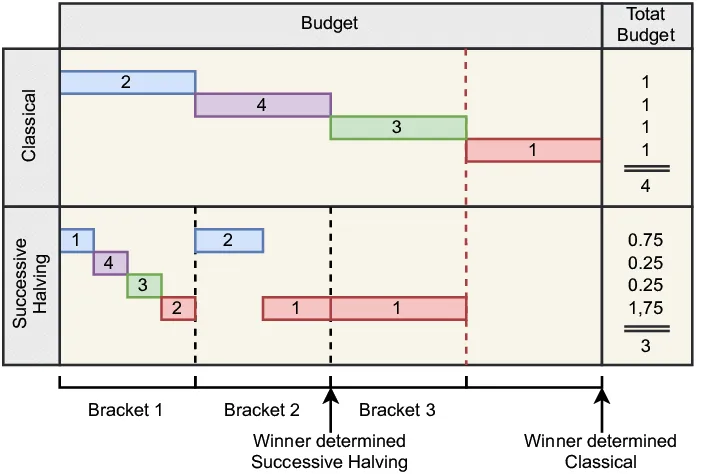
Successive Halving iteratively reduces the number of candidate configurations while increasing the resources allocated to the remaining candidates. It resembles a tournament where poorly performing candidates are eliminated and better ones receive more resources for further evaluation.

from sklearn.datasets import load_irisfrom sklearn.ensemble import RandomForestClassifierfrom sklearn.experimental import enable_halving_search_cv  # noqafrom sklearn.model_selection import HalvingGridSearchCVX, y = load_iris(return_X_y=True)clf = RandomForestClassifier(random_state=0)param_grid = {"max_depth": [3, None], "min_samples_split": [5, 10]}search = HalvingGridSearchCV(clf, param_grid, resource='n_estimators', max_resources=10, random_state=0).fit(X, y)search.best_params_

Method 7: LLM Chain-of-Thought for Hyperparameter Proposals

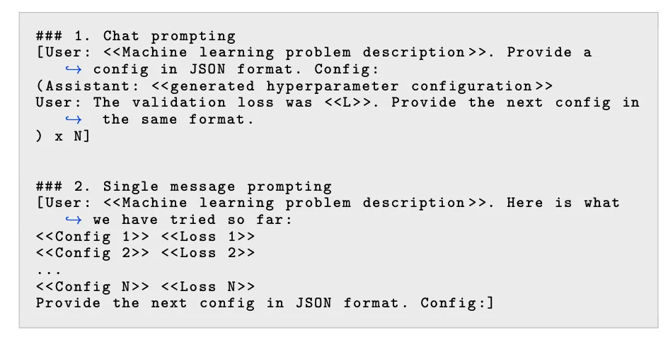
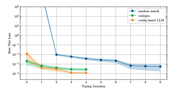
Large language models can be used to propose sets of hyperparameters for evaluation. After receiving a proposal, the model is trained with that configuration and the resulting metric, such as validation loss, is recorded. The process is iterative: the LLM is queried again to suggest the next configuration.

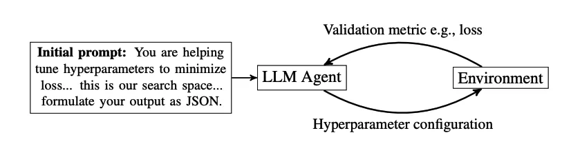
When used for hyperparameter optimization, LLMs can apply chain-of-thought reasoning to explain why a particular set of hyperparameters was recommended. This reasoning can help interpret the suggestions and provide deeper insight into the recommendations.