ALLPCB


Introduction
Face fusion refers to taking two input faces A and B and producing an output face C that shares features of both A and B. The output is a new synthetic face. The typical face-fusion pipeline has three steps: facial landmark detection, face fusion, and face swapping.
Step 1: Use a model trained with deep learning to detect key landmarks on the two input images.
Step 2: Fuse the faces according to the landmark results.
Step 3: Paste the fused face onto a target face and blend to form the final image.
In practice, completing step 2 already meets the basic requirements of face fusion. Face swapping is often used for generating synthetic faces and can have privacy implications if misused. Unrestricted swapping of real faces can lead to serious misuse, such as widespread deepfake videos.
1. Facial Landmark Localization
1.1 Training the model
Larger datasets produce more accurate models. A widely used dataset for facial landmark detection is 300-W (300 Faces In-The-Wild Challenge). In that challenge, teams detected faces and labeled 68 facial landmarks on each face. The dataset archive is large and contains many annotated faces. Training on such a dataset requires significant resources and time, so in this design a smaller dataset was used for training.
To train a landmark detector we used the imglab tool. Imglab is used to label images for training dlib or other object detectors. Example commands:
imglab -c training_with_face_landmarks.xml images imglab training_with_face_landmarks.xml
The first command creates an XML file that records the labels. The second command opens the imglab tool to label images. Following the dlib convention, label the 68 landmarks per image. Use shift+left-drag to select the face rectangle, double-click the rectangle, then use shift+left-click to add landmark points.
Next, start training the model. Training time depends on the computer performance. First, define the parameter settings function:
options = dlib.simple_object_detector_training_options()
Most parameters use defaults. For the smaller training set used here, the main parameter adjustments were:
- oversampling_amount: Randomly augment training samples. With N training images, the effective training count becomes N * oversampling_amount. A larger value yields more samples but increases training time. For a small dataset this example sets the value high (300).
- nu: Regularization parameter. Larger nu lets the model fit the training samples more closely.
- tree_depth: Tree depth. This example reduces model capacity by increasing regularization (smaller nu) and using shallower trees.
- be_verbose: Whether to print training progress. Set true to output training information.
1.2 Model testing
After training the landmark detector, evaluate its accuracy on both the training set and an independent test set. For the training-set accuracy:
print("Training accuracy{0}".format(dlib.test_shape_predictor(training_xml_path, "predictor.dat")))
For test-set accuracy:
print("Testing accuracy:{0}".format(dlib.test_shape_predictor(testing_xml_path, "predictor.dat")))
1.3 Landmark detection
Use the trained model to detect facial landmarks. Example usage:
predictor = dlib.shape_predictor("predictor.dat") dets = detector(img, 1) # returns face rectangles; use len(dets) for number of faces landmarks = [[p.x, p.y] for p in predictor(img1, d).parts()]
2. Face Fusion
This section introduces two core algorithms: Delaunay triangulation and affine transformation.
2.1 Delaunay triangulation
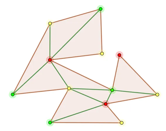
Let V be a point set. For edge e with endpoints x and y, if there exists a circle through x and y such that no other point in V lies inside that circle (the circle may pass through at most three points including x and y), then e is a Delaunay edge. If a triangulation T of V contains only Delaunay edges, it is a Delaunay triangulation.
Delaunay triangulation has two important properties. The empty circumcircle property: assuming no four points are cocircular, the circumcircle of any triangle in a Delaunay triangulation contains no other points. The max-min angle property: among all triangulations of a point set, Delaunay triangulation maximizes the minimum angle, producing more regular triangles.
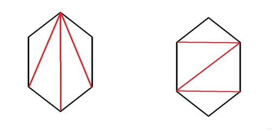
The algorithm conceptually relates to the art gallery problem: decompose a polygon into triangles to simplify coverage. In face fusion, Delaunay triangulation is used to split the face into triangles that will be individually transformed and blended.
OpenCV provides the Subdiv2D class for Delaunay triangulation. Example usage:
subdiv = cv2.Subdiv2D(rect) subdiv.insert(point) triangleList = subdiv.getTriangleList()
Draw the triangulation with cv2.line().
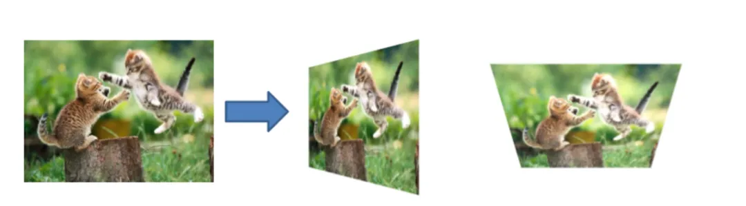
2.2 Affine transformation
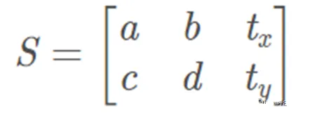
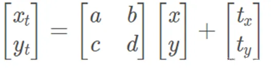
An affine transformation is a linear transformation followed by a translation. It preserves straightness and includes rotation, scaling, translation, and shear. An affine transform matrix is typically 2x3; the third column encodes translation. The transform maps a 2D coordinate (x, y) to (xt, yt).
Before applying affine transforms, preprocess the detected landmarks. Save the 68 facial landmarks for face A and face B locally. Because the faces to be fused may differ in size, compute an average set of landmarks to serve as the target positions for the fused face. After triangulation, the face is split into triangles. For each triangle, use the corresponding three points from face A and face B to form triangles A and B; the averaged triangle is C.
Only each triangle needs to be transformed rather than the whole image. Compute the bounding rectangle of the triangle to improve efficiency.
r = cv2.boundingRect(np.float32([t])) # r is a tuple: (x, y, w, h) tRect.append(((t[i][0] - r[0]), (t[i][1] - r[1])))
Create a mask for the triangle area with cv2.fillConvexPoly, then apply affine transforms to map triangle A and triangle B to triangle C.
Example calls for warping two triangle patches into the target triangle:
warpImage1 = applyAffineTransform(img1Rect, t1Rect, tRect, size) warpImage2 = applyAffineTransform(img2Rect, t2Rect, tRect, size)
The applyAffineTransform function uses cv2.getAffineTransform to compute the affine matrix and cv2.warpAffine to apply it:
# Apply affine transform calculated using srcTri and dstTri to src and output an image of size def applyAffineTransform(src, srcTri, dstTri, size): # Given a pair of triangles, find the affine transform. warpMat = cv2.getAffineTransform(np.float32(srcTri), np.float32(dstTri)) # Apply the Affine Transform just found to the src image dst = cv2.warpAffine(src, warpMat, (size[0], size[1]), None, flags=cv2.INTER_LINEAR, borderMode=cv2.BORDER_REFLECT_101) return dst
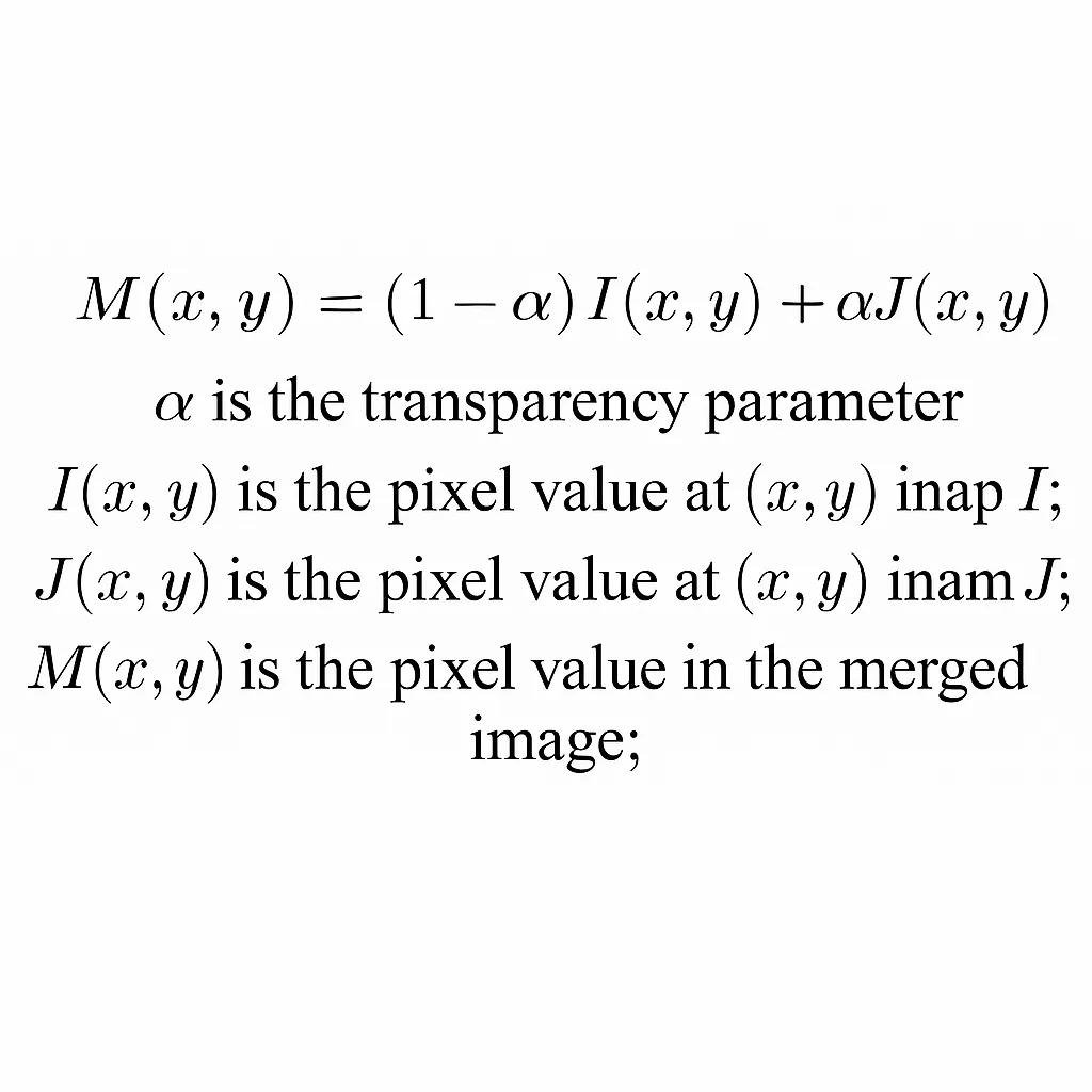
2.3 Image blending
After warping each triangle from both faces to the target triangle positions, blend the images by alpha compositing. If alpha is 0.5, both faces contribute equally:
imgRect = (1.0 - alpha) * warpImage1 + alpha * warpImage2
Finally, multiply the blended result by the triangle mask to keep only the triangle region and paste it into the output image. After processing all triangles, the fused face is obtained. The more accurate and dense the landmark points, the better the fusion result will be.
3. Face Swapping
Face swapping consists of five steps: landmark detection, finding the convex hull, triangulation based on the hull, affine warping, and seamless cloning. Landmark detection, triangulation, and affine warping were described above. The following focuses on convex hull computation and seamless cloning.
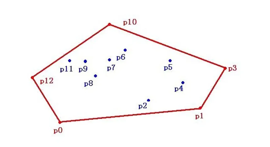
3.1 Convex hull algorithm
For a point set V on the plane, the convex hull is the smallest convex polygon that contains all points of V either inside or on its boundary. In face swapping, we compute the convex hull of the 68 landmarks to obtain a polygon enclosing the face area. OpenCV provides cv2.convexHull() to compute it.
Face swapping differs from face fusion in that it typically pastes face A onto face B directly. Therefore, working with the convex hull of the landmarks is sufficient: triangulate that polygon and warp triangles from A to B. The core warping code for triangles is shown below.
# Warps and alpha blends triangular regions from img1 and img2 to img2 def warpTriangle(img1, img2, t1, t2): # Find bounding rectangle for each triangle r1 = cv2.boundingRect(np.float32([t1])) r2 = cv2.boundingRect(np.float32([t2])) # Offset points by left top corner of the respective rectangles t1Rect = [] t2Rect = [] t2RectInt = [] for i in range(0, 3): t1Rect.append(((t1[i][0] - r1[0]), (t1[i][1] - r1[1]))) t2Rect.append(((t2[i][0] - r2[0]), (t2[i][1] - r2[1]))) t2RectInt.append(((t2[i][0] - r2[0]), (t2[i][1] - r2[1]))) # Get mask by filling triangle mask = np.zeros((r2[3], r2[2], 3), dtype=np.float32) cv2.fillConvexPoly(mask, np.int32(t2RectInt), (1.0, 1.0, 1.0), 16, 0) # Apply warpImage to small rectangular patches img1Rect = img1[r1[1]:r1[1] + r1[3], r1[0]:r1[0] + r1[2]] size = (r2[2], r2[3]) img2Rect = applyAffineTransform(img1Rect, t1Rect, t2Rect, size) img2Rect = img2Rect * mask # Copy triangular region of the rectangular patch to the output image img2[r2[1]:r2[1] + r2[3], r2[0]:r2[0] + r2[2]] = img2[r2[1]:r2[1] + r2[3], r2[0]:r2[0] + r2[2]] * ((1.0, 1.0, 1.0) - mask) img2[r2[1]:r2[1] + r2[3], r2[0]:r2[0] + r2[2]] = img2[r2[1]:r2[1] + r2[3], r2[0]:r2[0] + r2[2]] + img2Rect
3.2 Seamless cloning
Seamless cloning blends a selected region of a source image into a target image so that the result appears natural without visible seams. Traditional copy-paste or clone tools can leave visible edges when color or illumination differs between source and target. Seamless cloning addresses this by solving a Poisson equation constrained by the Laplacian inside the selected region and Dirichlet boundary conditions on the region border, which yields a unique solution.
In practice, compute the gradient fields of the source image A and background image B, replace the gradient field in the selected region with A's gradients, compute the divergence (b), and solve the linear system Ax = b for pixel values. Although the math can be involved, OpenCV provides a convenient function cv2.seamlessClone to perform the operation.
When the source face crop includes dark background around the face, seamless cloning can produce visible artifacts at the face boundary. To reduce such artifacts, include a coarse set of extra points around the face region (for example, eight additional points) so that surrounding context is also considered when blending. You can obtain image dimensions with:
sp = img1.shape # [height, width, channels]
Using this, choose points around the face to reduce seam artifacts caused by dark background and improve cloning results.
4. Experimental analysis and summary
In experiments fusing two faces of the same gender and similar appearance, the resulting fused face achieved high realism and met the expected objectives. When fusing faces of different gender and skin tones and swapping them onto male and female subjects, the algorithm still produced natural-looking results without noticeable artifacts in gender or skin tone.
When fusing faces of different sizes, the fused output remained realistic. One identified issue was illumination: a face with a shadow caused by lighting led to the shadow being interpreted as skin tone by the algorithm, so the fused result retained the shadow and looked slightly unnatural. Addressing illumination effects is a future direction.
Overall, the experiments demonstrate that the described face-fusion approach can produce realistic fused faces. Areas for improvement include:
- Eliminate the influence of lighting-induced shadows on fusion. Possible directions: preprocess images to reduce lighting effects, or handle shadow regions explicitly during fusion. Preprocessing is a more practical initial approach.
- Reduce the impact of occlusions such as hair and glasses. The current algorithm treats occlusions as part of the face and includes them in triangulation and warping, which can degrade results. As occlusions are common in real images, methods to detect and handle them will improve fusion robustness.