ALLPCB


Phased Array System Overview
The phased array system toolbox provides algorithms and applications for the design, simulation, and analysis of sensor array systems in radar, wireless communications, and medical imaging. The toolbox includes pulsed and continuous waveforms and signal processing algorithms for beamforming, matched filtering, direction-of-arrival (DOA) estimation, and target detection. It also includes models for transmitters and receivers, propagation, targets, jammers, and clutter.
Radar Data Sampling and the Radar Data Cube
In practice, the fast-time dimension (a single pulse) is often sampled at a rate higher than the Nyquist rate, producing a sequence of samples that form one record in the radar data cube. Multiple array elements receive data simultaneously on multiple channels.
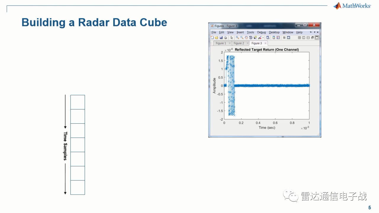
Figure 1: Fast-time samples for a single pulse
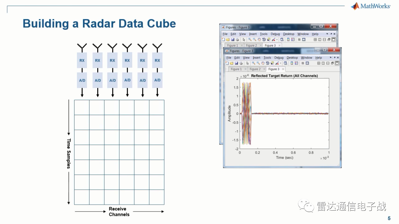
Figure 2: Received channel data across multiple array elements
Radars generally transmit periodic pulse trains. Often M pulses are processed as a coherent processing interval (CPI). Within a CPI, data collection typically uses a fixed PRI and carrier frequency, and the same radar waveform for each pulse.
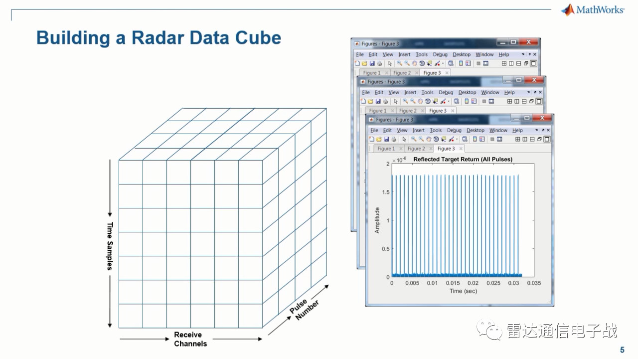
Figure 3: Slow-time data across multiple pulses
Thus, N channels, L samples per single pulse, and M pulses form the radar data cube. Processing this data cube yields target range, velocity, and azimuth information. Below, simulated data is used to design a phased array system and analyze its performance under different scenarios.
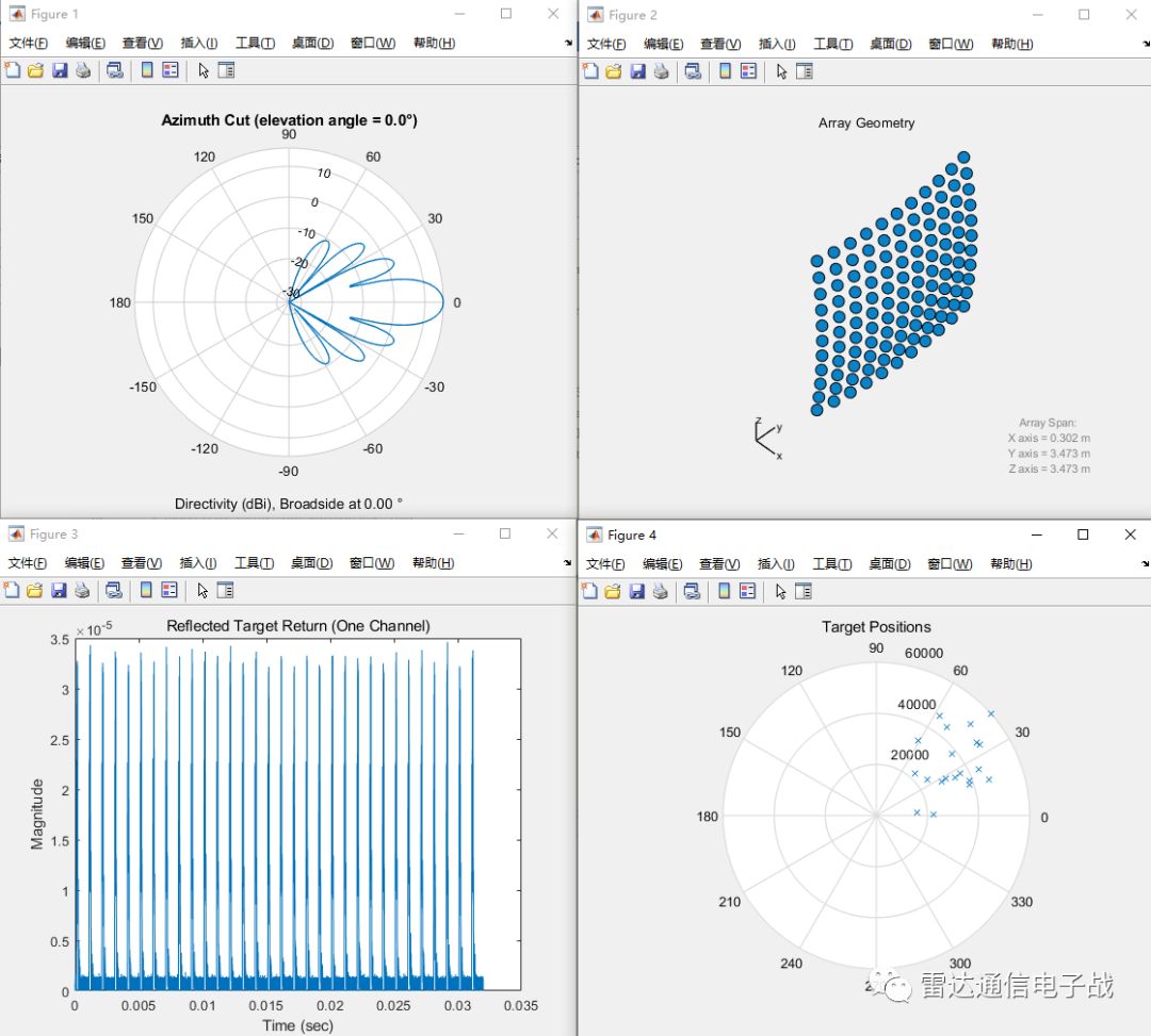
Figure 4: Simulation results for case 2
The accompanying video demonstrates generation of the radar data cube and the subsequent processing steps. Video source: MathWorks
Core Signal Processing Steps
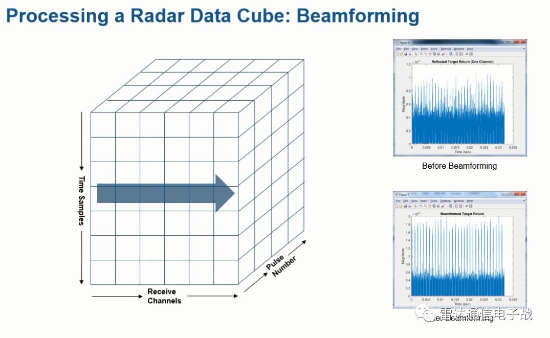
Figure 5: Beamforming
Processing across N receive channels is beamforming, processing L samples within a single pulse is pulse compression, and processing M pulses is Doppler processing. These correspond to azimuth, range, and velocity estimation, respectively.
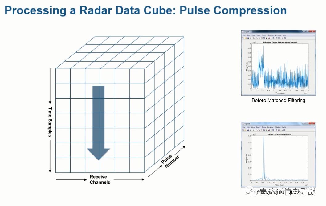
Figure 6: Pulse compression
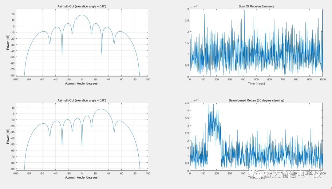
Figure 7: Doppler processing
Simulation results show that after beamforming, the signals from multiple channels coherently combine so that the echo emerges from noise and the signal-to-noise ratio is improved, followed by pulse compression and Doppler processing.