ALLPCB


Overview
This article analyzes the Kalman filter family and sliding-window optimization methods, and systematically reviews four classes of visual-inertial, LiDAR-inertial, visual-LiDAR, and LiDAR-visual-inertial SLAM fusion schemes and related open-source algorithms: algorithms.
01 State Estimation Algorithms
1.1 Kalman Filter Family
In SLAM, priors typically come from a set of sensors such as an inertial measurement unit (IMU) and encoders, while observations come from other sensors such as GPS, cameras, and LiDAR. The posterior is the result of fusing prior information with observations and represents the optimal pose estimate given all available information. It can be expressed as:
Here, x_k denotes the robot state vector at time k, including position and attitude; x_0 is the initial state vector; u_{1:k} represents inputs from time 1 to k; and z_{1:k} denotes all observations up to time k.
The Kalman filter (KF) is a common method for robot state estimation and is a leading technique in Bayesian filtering, but it is only applicable to linear Gaussian systems.
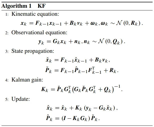
Kalman filter algorithm flowchart
Extension: EKF
The extended Kalman filter (EKF) is an important variant of KF that is suitable for handling nonlinear systems.
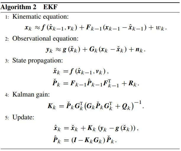
Extended Kalman filter algorithm flowchart
Iterated EKF (IEKF)
For nonlinear problems, the iterated EKF improves the linearization point through multiple iterations to reduce error. It repeatedly recomputes and updates the Kalman gain and state estimate until convergence or negligible change. This increases computation but can mitigate shortcomings of the standard EKF.
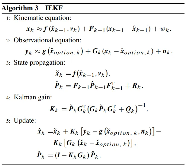
Iterated Kalman filter algorithm flowchart
Error-State Kalman Filter (ESKF)
The error-state Kalman filter is designed to better handle nonlinear problems. Compared with standard EKF, ESKF separates the true state and a nominal state and estimates the error as a state variable, which simplifies handling of nonlinearities.
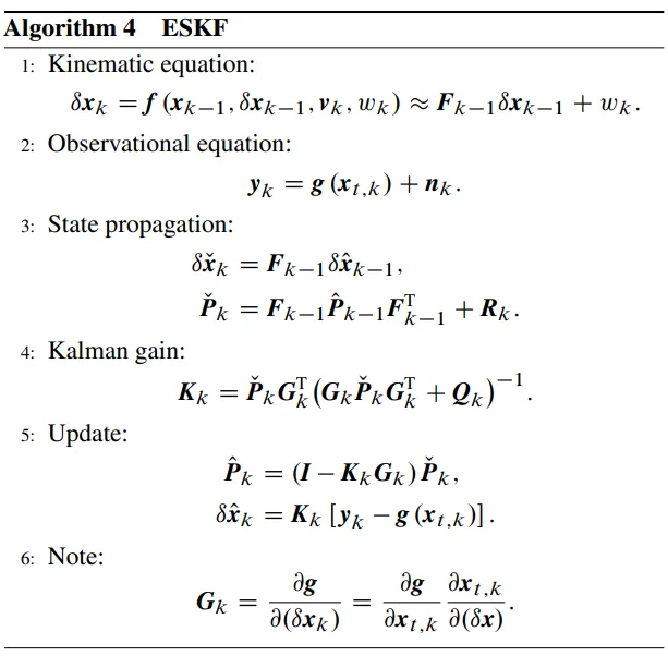
Error-state Kalman filter algorithm flowchart
1.2 Sliding-Window Optimization
Sliding-window optimization jointly optimizes all states inside a sliding window. For a window with n states, the optimal solution can be obtained by minimizing the following residuals:
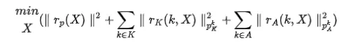
Here, r_imu is the residual derived from IMU preintegration; r_vloar is the residual from vision or LiDAR; P_imu and P_vloar are the corresponding covariance terms; Z_imu is the IMU measurement set; Z_vloar is the vision or LiDAR measurement set. r_prior is the prior residual retained after marginalizing the previous window.
02 Multisensor Fusion Algorithms
Multisensor fusion can be categorized into four groups: visual+IMU, LiDAR+IMU, visual+LiDAR, and visual+LiDAR+IMU. Representative state-of-the-art algorithms in each category are summarized below.
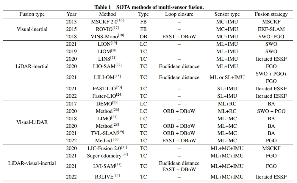
State-of-the-art multisensor fusion algorithms. Notes: (1) Type: FB-filter based, OB-optimization based, LC-loosely coupled, TC-tightly coupled. (2) Loop closure: FAST and ORB-feature points, DBoW-bag-of-words. (3) Sensor types: MC-monocular, ML-mechanical LiDAR, SL-solid-state LiDAR, RC-RGB-D camera. (4) Fusion strategies: FGO-factor graph optimization, BA-bundle adjustment, SWO-sliding-window optimization, PGO-pose graph optimization.
2.1 Visual and IMU Fusion
Filter-Based Methods
MSCKF: Uses an unstructured method to handle visual information by considering recent camera poses within a window and their associated feature observations. This allows efficient 6-DoF pose estimation in real time using static features without including all historical features in the filter state vector, avoiding quadratic growth in computation as the number of features increases.
MSCKF 2.0: Addresses inconsistencies in observability that arise when using continuously updated estimates for linearizing the measurement model. The improved MSCKF 2.0 uses the first-available estimate for each state when computing Jacobians to ensure correct observability properties.
Optimization-Based Methods
OKVIS: Incorporates IMU preintegration to integrate IMU measurements into relative motion constraints, avoiding repeated IMU propagation as states change. The system also introduces keyframes and only tracks and optimizes features on recent keyframes to improve real-time performance and efficiency.
VINS-mono: In monocular scenarios, initialization is a major challenge because scale is observable only with accelerometer excitation, meaning monocular VINS cannot initialize from a static start. VINS-mono addresses camera-IMU extrinsic calibration, initialization, and processing with a pipeline that includes preprocessing, initialization, nonlinear VIO optimization, loop closure, and global pose graph optimization.
2.2 LiDAR and IMU Fusion
Loosely Coupled Methods
LOAM: A classic 3D LiDAR SLAM method with modules for feature extraction, odometry estimation, and map building. LOAM updates pose by matching edge and planar points between consecutive scans. In high-speed motion scenarios, LOAM's accuracy degrades, and integrating IMU measurements can compensate for motion distortion, improving accuracy and robustness.
LION: Designed as a lightweight structure for low computational load, focusing on accurate and robust localization when vision is not available. By combining LiDAR point-cloud features with continuous high-frequency IMU measurements, especially during rapid motion, LION compensates for motion distortion inherent in LiDAR-only methods and enhances navigation accuracy and stability.
Tightly Coupled Methods
LIOM: Adopts ideas from visual-inertial fusion by processing consecutive LiDAR scans in a sliding-window fashion and jointly optimizing poses. LIOM uses IMU preintegration to correct point-cloud distortion caused by rapid motion, improving localization accuracy and stability.
LINS: Employs an iterated extended Kalman filter to refine estimates; the iterative form allows the system to approach the true state more closely and reduce linearization errors. LINS also considers algorithm formulation in the robot-centered coordinate frame to suit various applications.
Other relevant methods include LIO-SAM, LILI-OM, and the FAST-LIO series.
2.3 LiDAR and Vision Fusion
Loosely Coupled Algorithms
DEMO: First transforms LiDAR point clouds into the camera coordinate frame using estimated camera poses and generates a depth map. Newly observed points in front of the camera are added to the map. Map points are represented in spherical coordinates and stored in a 2D k-d tree indexed by two angular coordinates. For each image feature, depth can be obtained by projecting onto a plane patch formed by the three nearest neighbors from the k-d tree.
LIMO: Combines a monocular camera and LiDAR, using deep learning to identify and remove dynamic object features to prevent unreliable features from affecting ego-motion estimation. This reduces trajectory drift caused by mismatches with dynamic objects and improves localization accuracy after fusion.
Tightly Coupled Algorithms
V-LOAM: Exploits the higher camera frequency relative to LiDAR to obtain observable scale from a visual odometry module, which helps correct LiDAR point-cloud distortion. It models drift of visual odometry during a single scan to improve de-distortion, then matches corrected point clouds to the map to further optimize pose estimates.
TVL-SLAM: Uses precise timestamp synchronization to align visual frames and LiDAR scans, enabling tightly coupled state estimation via factor graph optimization. By jointly considering visual features and LiDAR geometry, it reduces errors from independent sensor operation and improves robustness to dynamic objects, illumination changes, and textureless regions.
2.4 LiDAR, Vision, and IMU Fusion
Loosely Coupled Algorithms
VIL-SLAM: Uses a stereo camera as the visual sensor and can perform well in degraded scenes such as long tunnels where pure LiDAR systems may fail. The algorithm tightly integrates stereo matching and IMU measurements and uses fixed-lag smoothing to produce VIO pose estimates at IMU and camera rates. These estimates are used to remove motion distortion and register LiDAR point clouds to the map.
Tightly Coupled Algorithms
LIC-Fusion 2.0: Predicts motion using IMU measurements, refines estimates with a visual-inertial odometry, and then fine-tunes using LiDAR scan-to-map matching. LIC-Fusion 2.0 also introduces a plane feature tracking method that extracts planar points from IMU-dewarped LiDAR point clouds and uses a data association strategy within a sliding window that includes outlier rejection criteria, enabling efficient and robust LiDAR processing.
Super odometry: Uses an IMU-centric processing pipeline composed of three parts: IMU odometry, visual-inertial odometry, and LiDAR-inertial odometry. IMU biases are constrained by visual-inertial and LiDAR-inertial priors, while LiDAR-inertial odometry receives motion predictions from the IMU odometry. A dynamic octree structure supports real-time efficiency. The underlying insight is that if other sensors constrain IMU bias drift well, IMU-based estimates remain accurate because IMU data is noisy but rarely contains large outliers.
Other systems include LVI-SAM and R3LIVE.
03 Future Research Directions
Universal, Efficient Sensor Fusion Frameworks
Current advanced fusion frameworks are often designed for specific platforms, making deployment on other platforms with similar sensors difficult. There is a need for flexible and efficient fusion frameworks that can adapt to varied platform requirements and configurations.
Deep Learning in SLAM
Apply deep learning for improved feature extraction, noise suppression, dynamic object detection, and pose estimation.
Distributed Collaborative Approaches
Multiple robots equipped with different sensor types can collaborate on the same SLAM task, significantly reducing the workload of individual robots.