ALLPCB


Introduction
This article provides a broad overview of hardware and systems used to implement computer vision. It emphasizes breadth over depth, points readers to instructive references, and includes runnable source code. We begin with how images are formed, then cover pinhole cameras, lenses, sensors (CCD and CMOS), Bayer filters, and color reconstruction.
Imaging History
Photography projects a 3D scene onto a 2D plane. A pinhole camera achieves this projection with a small aperture in a dark chamber. Light passing through the aperture creates a sharp projection that artists could trace, but the image is dim because the pinhole collects little light.
Athanasius Kircher's 1645 engraving of a portable camera obscura from Ars Magna Lucis Et Umbrae
Pinhole cameras still attract interest today because they can capture striking images anywhere. Their drawback remains low brightness and long exposure times.
To collect more light, lenses were introduced. Placing a lens in front of the aperture concentrates light and can change the magnification of the projected image. Modern zoom works by moving lens elements to change magnification without changing the distance between scene and image plane.
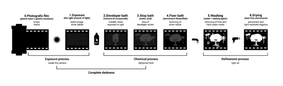
In the 1830s, Louis Daguerre introduced photographic plates that recorded light physically on a surface coated with silver halide. Exposed silver halide converts to metallic silver; after chemical development, the latent image becomes visible. This made it possible to record a moment by pressing a shutter instead of tracing the projection by hand.

The invention of silicon-based image detectors had an even larger impact than film. The same silicon chips can capture an essentially unlimited number of images without chemical development. These detectors are the basis of digital cameras and the cameras in most smartphones.
Image Sensors
In essence, photography maps a 3D scene to a 2D plane. The aperture performs the projection, lenses gather light and adjust magnification, and the image plane evolved from a drawing surface to silver-halide film and finally to silicon image sensors.
Most image sensors convert incoming photons to a digital image by exploiting silicon's properties. A photon with sufficient energy striking a silicon atom frees electrons. Photon flux at a pixel generates an electron flux; that charge is then converted to a voltage.
Charge-Coupled Device (CCD)
In CCD sensors, photon-to-electron conversion occurs at each pixel. A capacitor under each pixel stores the freed electrons. A vertical CCD shift register connects capacitors in each column, allowing charges to be shifted down one pixel at a time until they reach the last row. A horizontal CCD shift register then moves charges to an analog-to-digital converter (ADC).
Vertical transfer in CCDs uses a bucket-brigade approach: each row transfers its charge to the next row. Horizontal transfer preserves row order; when charges reach the ADC they are converted to voltages proportional to their charge.
Complementary Metal-Oxide-Semiconductor (CMOS)
CMOS sensors implement image capture differently. Instead of transferring electrons from pixels to an ADC, CMOS integrates voltage conversion at the pixel level.
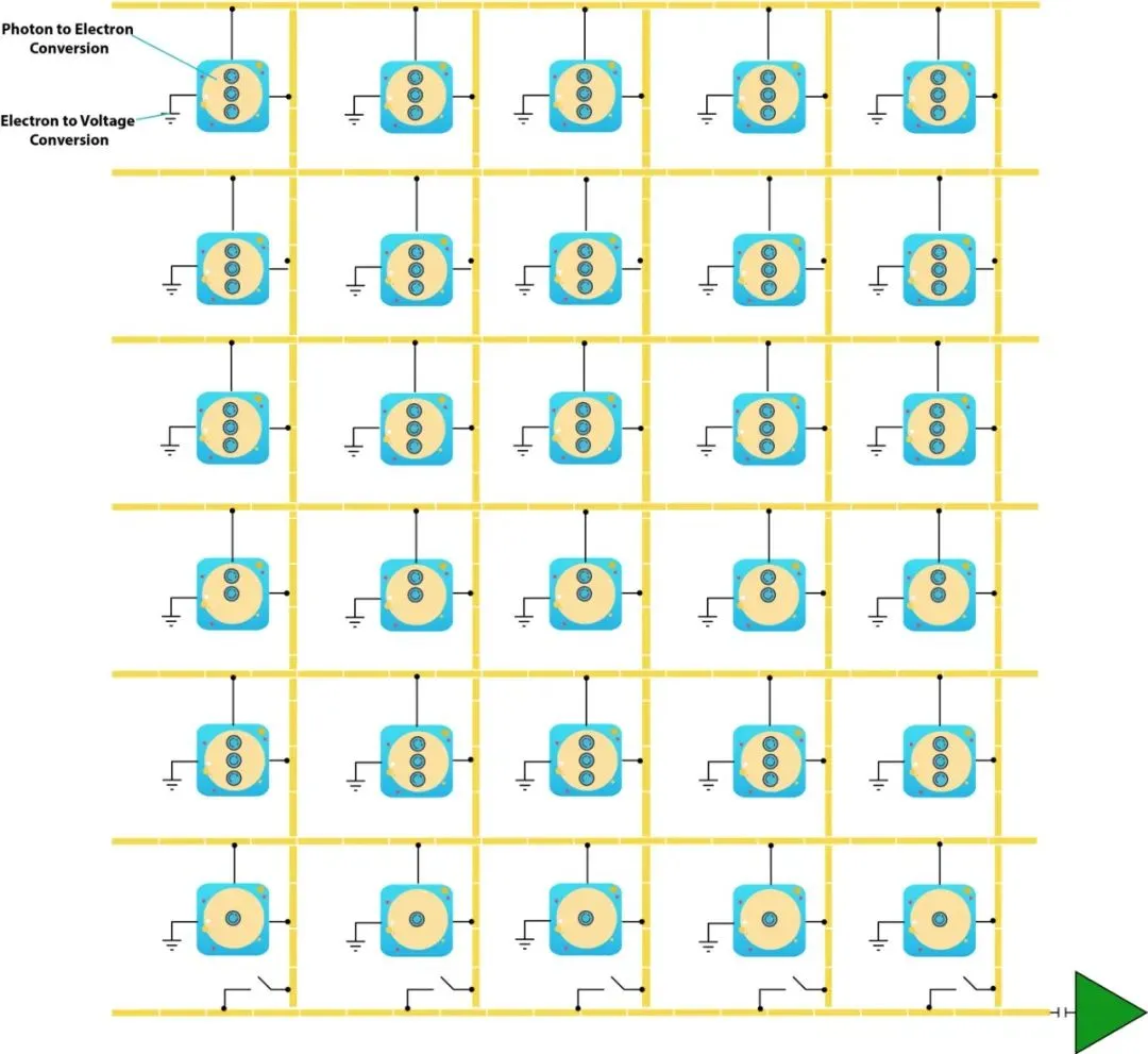
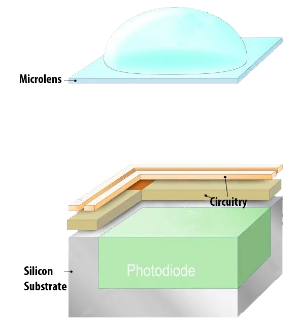
CMOS allows individual addressing of pixels to read their voltages, providing flexibility such as faster readout of regions of interest. That flexibility comes at the cost of a smaller photosensitive area per pixel because more circuitry is integrated at the pixel. Microlenses are often placed above each pixel to focus light onto the photosensor and mitigate reduced light collection.
Color Capture
Pixels directly measure light intensity but not wavelength. To capture color, the most common approach is a Bayer color filter array in which each pixel is covered by a red, green, or blue filter.
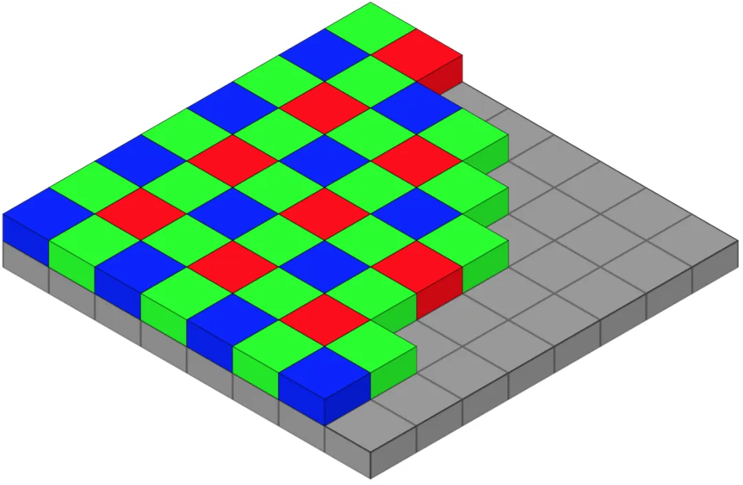
A 2×2 Bayer cell contains two green, one blue, and one red filter. Human color perception can be approximated with three wavelength bands, so capturing R, G, and B is sufficient to reproduce perceived colors. A raw Bayer image, however, stores only one color channel per pixel and therefore appears mosaic-like and biased toward green because the pattern has twice as many green filters.
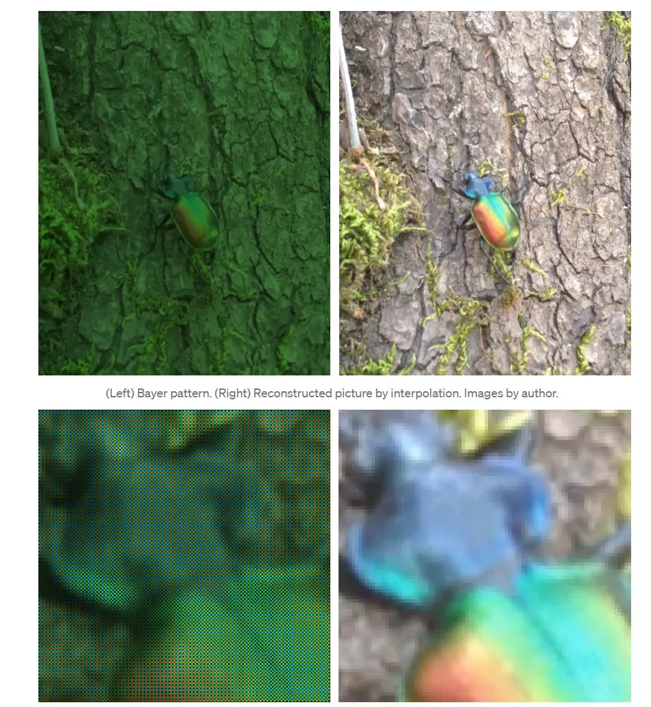
Demosaicing converts the raw Bayer image into a full-color image by interpolating each pixel's missing color components from neighboring pixels.
Computer Vision
Image sensors are fundamental components in many applications, shaping how we communicate and opening interdisciplinary fields. One of the most advanced of these fields is computer vision.
Studying computer vision requires an appreciation for the underlying hardware. After a brief review of hardware, we now examine a practical application that uses these sensors.
Lane Detection in Autonomous Driving
Starting in May 2021, Tesla began delivering some Model 3 and Model Y vehicles without radar. Those models rely on camera-based autonomy to provide equivalent functionality under the same safety rating.
One safety feature in camera-based systems is lane departure warning/avoidance. Detecting road lanes is essential for driving. Below we implement lane detection two ways: first using classical computer vision algorithms, then using convolutional neural networks.
Edge Detection
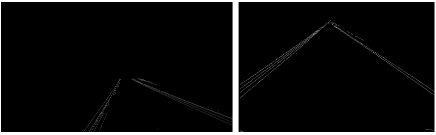
The first step is detecting prominent edges in the image. Regions with large differences in intensity between adjacent pixels are marked as edges. The code below converts the image to grayscale, applies a Gaussian blur to reduce noise, and uses the Canny edge detector.
def canny(image):
    gray = cv2.cvtColor(image, cv2.COLOR_RGB2GRAY)
    blur = cv2.GaussianBlur(gray, (5, 5), 0)
    canny = cv2.Canny(blur, 10, 30)
    return canny
These edge images contain much information that is not relevant. To focus on the road ahead, define a polygonal region to mask each image. The polygon points differ between images depending on perspective; drawing the image and checking width and height helps determine appropriate coordinates.
def region_of_interest(image):
    height = image.shape[0]
    width = image.shape[1]
    polygons = np.array([[(10, height), (width, height), (width, 1100), (630, 670), (10, 1070)]])
    mask = np.zeros_like(image)
    cv2.fillPoly(mask, polygons, 255)
    masked_image = cv2.bitwise_and(image, mask)
    return masked_image

Within the masked region, lane lines appear as sequences of pixels that the human eye perceives as lines. To track the main lines that best describe these pixel arrangements, use the Hough transform.
lines = cv2.HoughLinesP(cropped_image, 2, np.pi/180, 100, np.array([]), minLineLength=40, maxLineGap=5)
This classical approach can work well but has limitations:
- The region of interest must be defined explicitly for each case. Due to perspective changes, a single polygon mask cannot cover all situations.
- Computation can be too slow for real-time driving without sufficient processing power.
- Curved lanes are not well represented by straight-line Hough detections.
Conclusion
Understanding imaging hardware—how images are formed, captured, and processed—is important for developing computer vision systems. Classical algorithms provide insight and simple implementations, while modern neural approaches address some limitations but require additional considerations.