ALLPCB


Overview
Ultrasound systems are among the most precise and complex signal-processing instruments in widespread use. As with any complex instrument, many trade-offs are required during implementation because of performance, physical, and cost constraints. System-level knowledge is necessary to understand the required functionality and performance level of the front-end ICs, especially low-noise amplifiers (LNA), time-gain compensation amplifiers (TGC, a type of variable gain amplifier), and analog-to-digital converters (ADC). These analog signal-processing ICs largely determine overall system performance. The characteristics of the front-end ICs set system performance limits; once noise and distortion are introduced, they cannot practically be removed.
System architecture and channel count
Typical systems terminate relatively long cable bundles (about 2 m) with microcoaxial conductors, commonly 48 to 256 channels, at a multi-element sensor array. Some arrays use high-voltage multiplexers or demultiplexers to reduce the complexity of transmit and receive hardware at the expense of flexibility. The most flexible approach is phased-array digital beamforming, which requires full electronic control of all channels and is often the most costly to implement. Advances in front-end components such as dual and quad variable-gain amplifiers and multi-channel ADCs have reduced per-channel cost and power requirements, making full electronic control of all channels feasible even for mid-range systems.
Transmit and receive front end
On the transmit (Tx) side, the transmit beamformer determines the delay pattern required to set the desired transmit focus and drives the transmit amplifier, which provides the high voltage needed to excite the sensor elements. On the receive (Rx) side, a transmit/receive (T/R) switch isolates the receiver from the high-voltage Tx pulse; this switch is commonly implemented with diode bridges that isolate the Tx pulse and are followed by an LNA and one or more VGAs.
Beamforming and image formation
After amplification, either analog beamforming (ABF) or digital beamforming (DBF) is performed. Apart from continuous-wave (CW) Doppler processing, which has a dynamic range too large for standard imaging channels, most current imaging systems use DBF. Finally, the received beam is processed to generate gray-scale images, two-dimensional color images, and/or color Doppler outputs.
The primary aims of an ultrasound system are accurate imaging of internal anatomy and characterization of blood flow using Doppler processing. The following sections analyze the technical challenges related to signal attenuation, power consumption, and dynamic range, and discuss the front-end IC selection considerations for meeting those challenges.
1. Signal attenuation
Ultrasound acquisition modes include B-mode (brightness or gray-scale imaging, 2D), F-mode (colorflow imaging or Doppler imaging for blood-flow detection), and D-mode (spectral Doppler).
Medical ultrasound operates from about 1 MHz to 40 MHz. External imaging commonly uses 1 MHz to 15 MHz, while devices for superficial vessels may use frequencies up to 40 MHz. Tissue attenuation is frequency dependent and is approximately 1 dB/cm/MHz. For example, a 10 MHz signal at 5 cm penetration experiences a round-trip attenuation of roughly 1 dB/cm/MHz × 5 cm × 2 × 10 MHz = 100 dB.
This large attenuation imposes a strict requirement on receiver dynamic range: the receive circuitry must achieve very low noise while also handling large signals, and it must recover from overloads rapidly. The T/R switch must prevent large transmit pulses from saturating the receiver; leakage of even a small portion of the transmit energy can overload the receiver. Poor overload recovery leaves the receiver blinded until it recovers, which directly affects the minimum imaging depth from the skin surface.
2. ABF and DBF systems
Both analog beamforming (ABF) and digital beamforming (DBF) operate by delaying or storing the received pulses from each channel so they align in time for a given focus, then coherently summing them. This coherent summation provides spatial processing gain because the signal is coherent across channels while noise is uncorrelated, yielding a theoretical processing gain of 10·log10(N), where N is the number of channels.
There are two implementation approaches. In ABF, analog delay lines provide the required delays, the analog signals are summed, and a single high-resolution, relatively low-speed ADC digitizes the summed signal after downconversion. In DBF, the analog signal from each sensor element is digitized as close to the array as practical, stored in memory (FIFO), and then digitally delayed and summed. Both approaches demand excellent inter-channel matching. Both require VGAs, but DBF requires many high-speed, high-resolution ADCs because it samples RF-band signals at or near the sensor elements, whereas ABF needs only a single ADC after the analog summation and downconversion.