Multi-Sensor Spatial-Temporal Calibration Techniques

Overview

Extrinsic calibration and time synchronization of multiple sensors (collectively referred to as spatial-temporal calibration) are prerequisites for sensor fusion. Previous fusion discussions typically assume calibration has already been completed. In practice, calibration must be done before fusion. It is discussed later here because calibration involves more concepts than fusion; alternatively, calibration can be viewed as a higher-level form of fusion.

Because there are many calibration methods and many different calibration targets, this article will not cover every method in full detail. Instead, it summarizes common approaches and clarifies which type of method is appropriate in different situations. Details can be studied when a specific method is needed.

1. Extrinsic Calibration Methods

Compared with time calibration, extrinsic calibration is somewhat simpler, so it is introduced first.

The distinction between methods that do or do not have co-visibility is important because they are fundamentally different in principle and accuracy. In practice, sensors are often arranged to provide co-visibility when possible.

1. Radar and Camera Extrinsic Calibration

For this class of tasks, the PnP-based approach is commonly used.

Detaile d formulas and implementation can be found in the papers and code. Here is an intuitive description of the principle. When a camera and lidar have co-visibility, both can observe the calibration target and extract features such as edges or points. A residual model is built to describe the distance between corresponding features across the sensors. The residuals are functions of the extrinsic parameters, so optimizing to minimize the residuals yields the extrinsic transformation between the sensors.

2. Multi-LiDAR Extrinsic Calibration

The core idea of these methods is to extract planar features from each lidar's point cloud. In theory, with correct extrinsics, the same plane measured by multiple lidars should coincide when transformed into a common frame. If they do not coincide, the misalignment indicates extrinsic error. Using the plane mismatch as the residual and the extrinsic parameters as variables, an optimization problem can be formed and solved to estimate the extrinsics.

3. Hand-Eye Calibration

The term hand-eye calibration originally referred to calibrating a camera mounted on a robotic manipulator. The same principle applies to any pair of sensors that do not share co-visibility but can each estimate their own pose, for example camera-to-IMU, lidar-to-IMU, or camera-to-lidar calibration.

The method is based on a single equation:

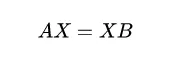
In this equation, X is the extrinsic transformation to be estimated, and A and B are the relative poses estimated independently by the two sensors. Combined with the diagram, the formulation should be clear.

Related references:

• Paper: LiDAR and Camera Calibration using Motion Estimated by Sensor Fusion Odometry
• Code: (code reference removed)

4. Calibration Within Fusion

As covered in previous articles, the fusion model is well understood. Calibration within fusion means including extrinsic parameters as part of the state vector in the fusion estimator and jointly estimating them with other states. With more variables, requirements for observability and the amount of information increase, which is why calibration can be seen as a higher-level fusion problem.

One practical advantage of in-fusion calibration is online calibration: extrinsics are estimated during normal operation without a separate calibration step. Many VIO/LIO systems implement this idea, including several well-known systems. Because these are established works, individual papers and code links are not listed here.

2. Time Calibration Methods

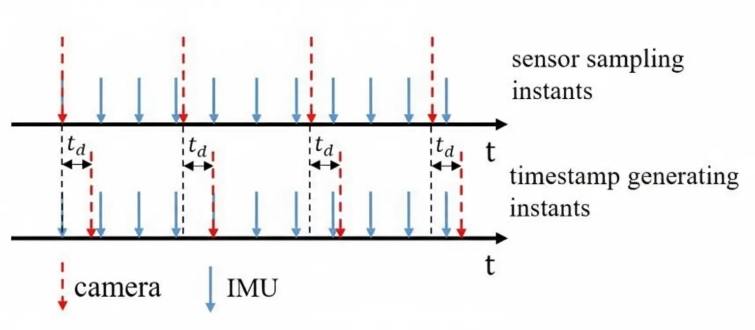
In many systems, each sensor uses its own clock, and because clocks are not synchronized, it is necessary to estimate time offsets between them. This is referred to as time calibration.

Time calibration is complex and difficult to do accurately. In practice, hardware solutions are preferred, for example using a common clock source for multiple sensors or applying a common timestamp to all sensors. Time calibration by algorithm is a fallback when hardware synchronization is not possible, such as in some mobile devices. Algorithmic time calibration incurs accuracy costs and is generally used only when hardware synchronization cannot be implemented.

Algorithmic time calibration approaches can be classified into discrete-time methods and continuous-time methods.

1. Discrete-Time Methods

Discrete-time methods address synchronization within the existing discrete-time fusion framework.

Two well-known approaches are described below.

1. Approach 1

   A study from HKUST applied to VINS is described in the paper Online Temporal Calibration for Monocular Visual-Inertial Systems.

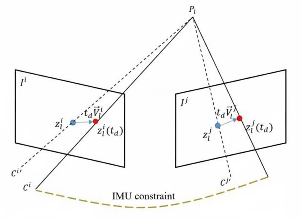
   The idea is clever: keep the IMU timestamps unchanged and adjust image feature positions based on a constant velocity motion model (illustrated below). The overall architecture remains the same, and with minimal changes the expected effect is achieved compared with ignoring time offsets.

   

2. Approach 2

   The second approach adjusts the integration interval according to the time offset when computing the camera pose in a filter. This is presented in the paper Online Temporal Calibration for Camera-IMU Systems: Theory and Algorithms.

   The corresponding state includes the time offset.

   

   The camera pose estimation model then becomes:

    

2. Continuous-Time Methods

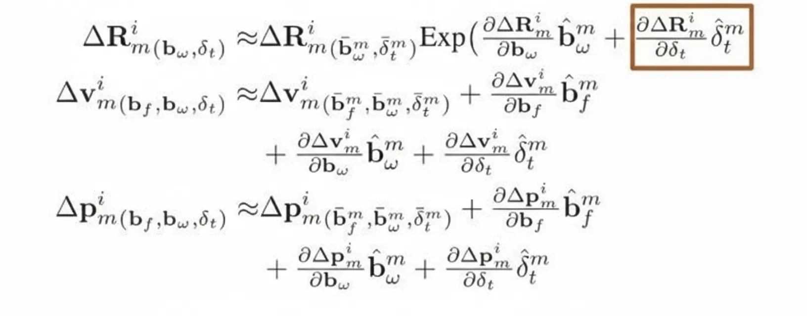
Continuous-time methods model inputs (accelerations, angular velocities) as continuous functions of time instead of discrete-time samples. When treating time offset as a state in preintegration, the interpolation function must be differentiable to obtain Jacobians; therefore continuous-time models are used so the interpolation is continuous and differentiable. The residuals and Jacobians are derived accordingly.

Because the time offset appears in Jacobians, differentiable interpolation functions are required, leading to the following Jacobian expression:

The remaining steps follow standard optimization procedures to solve the problem.

Continuous-time SLAM is a broad topic that cannot be fully covered here. Relevant works include:

• kalibr series
• Paper: Continuous-Time Batch Estimation using Temporal Basis Functions
• Paper: Unified Temporal and Spatial Calibration for Multi-Sensor Systems
• Paper: Extending kalibr: Calibrating the Extrinsics of Multiple IMUs and of Individual Axes
• Code: (code reference removed)

Other related work:

• Paper: Targetless Calibration of LiDAR-IMU System Based on Continuous-time Batch Estimation
• Code: (code reference removed)

Summary

Practitioners know that theoretical derivations do not always match empirical performance, so methods should be prioritized when chosen.

For extrinsic calibration, a rough ordering of accuracy from highest to lowest is:

1. Co-visibility based calibration
2. Calibration within fusion
3. Hand-eye calibration

Therefore, when high-precision methods are available, lower-precision methods should be avoided.

For time calibration, hardware synchronization should be used whenever possible. Algorithmic time calibration should be used only when hardware synchronization is not feasible, and time-offset estimation should be performed in environments with rich features.