ALLPCB


In the world of machine learning, accuracy is essential. You may tune and optimize parameters to improve a model, yet it rarely reaches 100% accuracy. This is the reality for predictive or classification models: they cannot achieve zero error. This article explains why this occurs and what other factors affect error.
Problem setup
Assume we observe a response variable Y (qualitative or quantitative) and an input vector X with p features or columns (X1, X2, ... , Xp). Suppose there is a relationship between them, which can be written as
f(X) = Y + e
Here f is some fixed but unknown function of X1, ..., Xp, and e is a random error term that is independent of X and has mean zero. In this expression, f represents the systematic information that X provides about Y. Estimating this relationship or f(X) from data is known as statistical learning.
In general, we cannot estimate f(X) perfectly, which leads to an error term called the reducible error. Improving the estimate of f(X) reduces the reducible error and thus increases model accuracy. However, even with a perfect estimate of f(X), the model will still incur error from e; this is the irreducible error in the equation, which we discussed above.
Put another way, the irreducible error captures variation that X cannot explain about Y. The term e may include useful predictor variables that were not measured: because they are not observed, f cannot use them for prediction. The term e may also include inherently unmeasurable variability. For example, for a given patient on a given day, the risk of an adverse reaction might vary due to manufacturing variability in the drug or the patient's general condition that day.
Such irreducible factors exist for every problem, and the associated error cannot be eliminated because these factors are typically not present in the training data. What we can do is reduce other forms of error to obtain an almost-perfect estimate of f(X). First, however, we need to review other important concepts in machine learning necessary for further understanding.
Model complexity
The complexity of the relationship f(X) between inputs and responses in a dataset is an important consideration. Simple relationships are easy to interpret. For example, a linear model has the form
Y = β0 + β1X1 + β2X2 + ... + βpXp
This representation makes it straightforward to infer how a specific feature affects the response. Such models are restrictive because they can only take a specific form—in this case, linear. But a true relationship might be more complex: it could be quadratic, circular, or take other forms. Flexible models can fit data more closely and often yield higher accuracy, but this flexibility comes at the cost of interpretability because complex relationships are harder to explain.
Choosing a flexible model does not always guarantee higher accuracy. A flexible statistical learning method may overfit the training data by capturing patterns that arise from random chance rather than from the true function f. This distorts the estimate of f(X) and leads to poorer generalization; this phenomenon is called overfitting.
When the goal is inference, simple and relatively inflexible statistical methods have clear advantages. In situations where prediction is the only objective and interpretability is not a priority, more flexible methods are often used.
Fit metrics
To quantify how close predicted responses are to observed responses for given observations, the most common metric in regression settings is the mean squared error (MSE).
MSE is the average of the squared differences between predictions and observations. When computed on the training data, it is the training MSE; when computed on unseen data, it is the test MSE.
For a given x0, the expected test MSE can be decomposed into three terms: the variance of the estimate of f(x0), the squared bias of the estimate of f(x0), and the variance of the error term e. The variance of e is the irreducible error discussed earlier. We will now examine bias and variance in more detail.
Bias
Bias refers to error introduced by approximating a possibly complex real-world relationship with a much simpler model. Thus, if the true relationship is complex and you try to use linear regression, you will certainly introduce bias in estimating f(X). No matter how much data you have, if you apply a simple algorithm in the presence of a complex true relationship, accurate predictions are impossible.
Variance
Variance measures how much the estimate of f(X) would change if it were derived from different training datasets. Because statistical learning methods are fit to the training data, different training samples will yield different estimates. Ideally, the estimate of f(X) should not vary much across different training sets. However, a high-variance method produces estimates that vary substantially with small changes in the training data.
General rule for bias and variance
Any change in the dataset provides a different estimate. If a statistical method matches the training data too closely, those estimates will fit the training observations well. A general rule is that when a method tries to match data points more closely or when a more flexible method is used, bias decreases but variance increases.
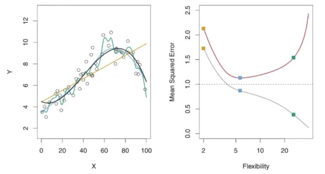
The figure above illustrates three regression methods. The yellow curve is a linear model, the blue curve is slightly nonlinear, and the green curve is highly nonlinear or very flexible, overfitting the data. On the right, the plot shows flexibility versus MSE: the red curve represents test MSE and the gray curve represents training MSE. The method with the lowest training MSE does not necessarily have the lowest test MSE, because some methods minimize training MSE at the cost of higher test MSE. This is an overfitting issue. As shown, the highly flexible green curve achieves the lowest training MSE but not the lowest test MSE.
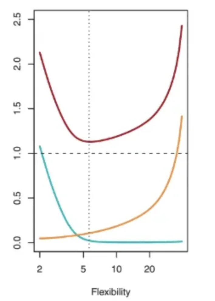
The next figure shows how test MSE (red curve), bias (green curve), and variance (yellow curve) change with model flexibility for a specific dataset. The optimal point for lowest MSE reflects a tradeoff between the two error forms. Initially, increasing flexibility reduces bias faster than it increases variance. After a certain point, bias stops decreasing while variance starts to increase rapidly due to overfitting.
Model flexibility corresponds to complexity: higher flexibility implies a more complex model.
Bias-variance tradeoff
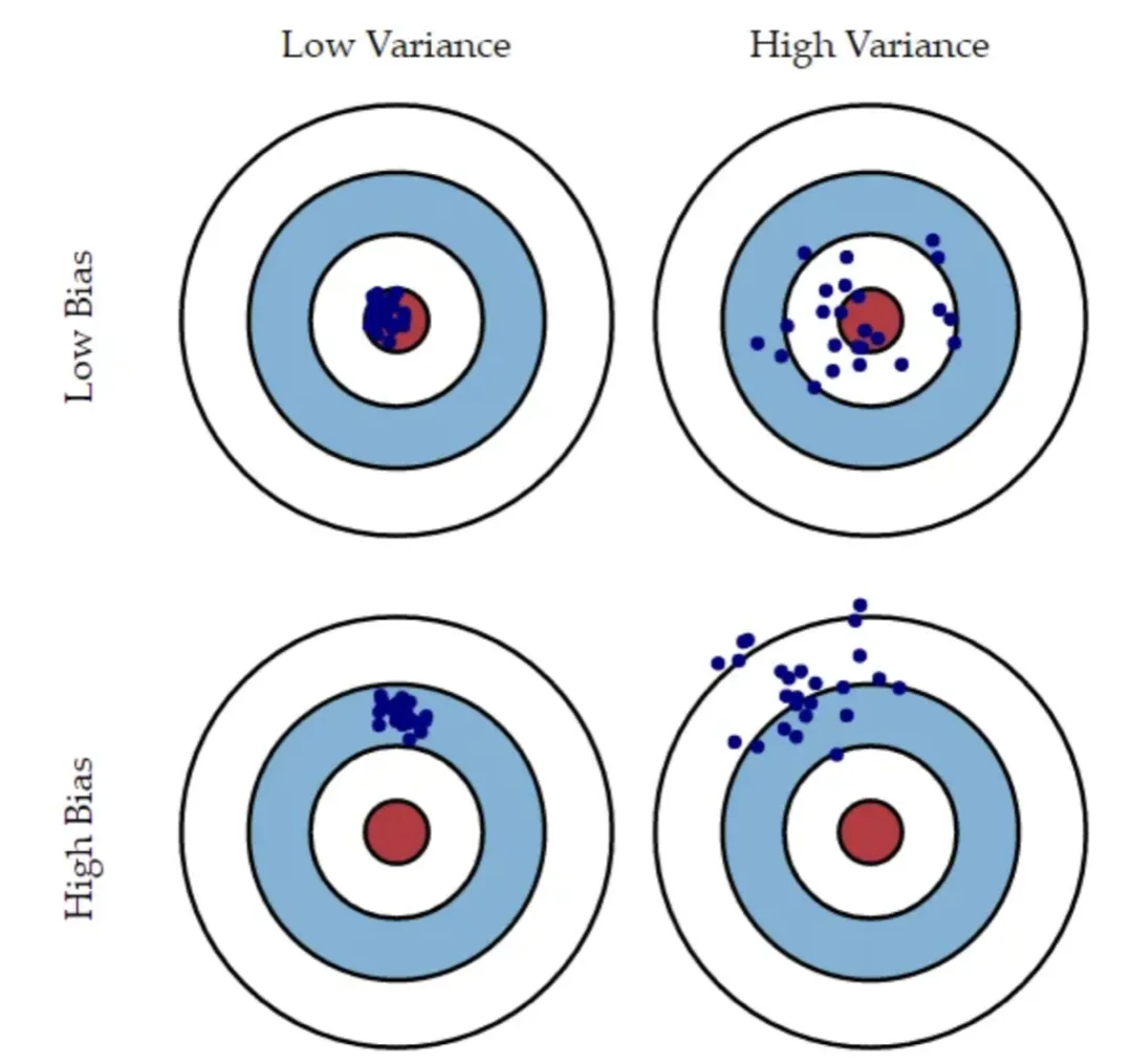
In the diagram above, imagine the bullseye represents a perfect model that predicts the true values. As points move away from the center, predictions worsen. If the model-building process is repeated many times on different datasets, each blue point represents the model obtained for the same problem from a different dataset. The diagram shows four situations combining high/low bias and high/low variance. High bias means the points are all far from the center; high variance means the points are widely dispersed.
The four quadrants illustrate: low bias and low variance; low bias and high variance; high bias and low variance; and high bias and high variance.
As discussed, to minimize expected test error we need a method that achieves both low variance and low bias. There is always a tradeoff because it is easy to obtain a method with very low bias but very high variance (for example, fitting a curve through every training point) or a method with very low variance but high bias (for example, fitting a horizontal line). The challenge is to find a method with both low variance and low squared bias.
Balancing bias and variance is essential for successful machine learning and is a key consideration during model development. Keeping this tradeoff in mind helps select an appropriate method for a given situation and improves predictive performance.