ALLPCB


In routine research, we often use statistical probability concepts to support urban studies. Therefore, mastering statistical probability topics is necessary. This article discusses commonly encountered probability distributions and aims to provide a conceptual overview.
1. Random variables
All possible outcomes of a random experiment are random variables. A set of random variables is denoted by X. If the possible outcomes are countable, the variable is called a discrete random variable. For example, if you flip a coin 10 times, the number of heads can be represented by an integer. The number of apples in a basket is also countable.
Continuous random variable
These are values that cannot be represented discretely. For example, a person might be 1.7 m tall, 1.80 m tall, 1.6666666... m tall, and so on.
2. Density functions
We use density functions to describe the probability distribution of a random variable X.
PMF: probability mass function
The PMF returns the probability that a discrete random variable X equals x. The sum over all possible values equals 1. The PMF applies only to discrete variables.
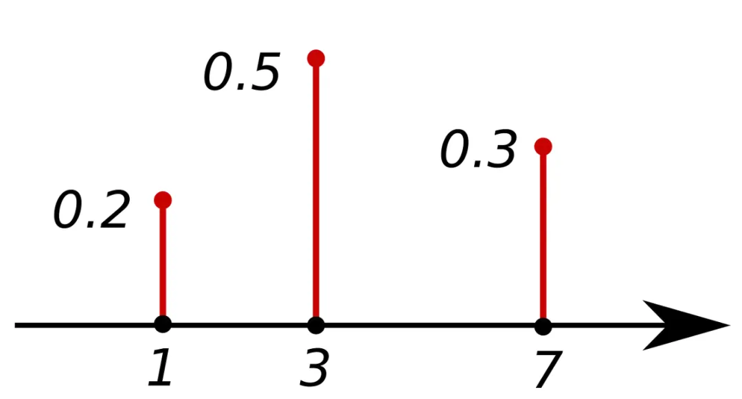
PMF. Source: Wikipedia
PDF: probability density function
The PDF is the continuous-variable counterpart to the PMF. It gives the probability for a continuous random variable X to fall within a given range.
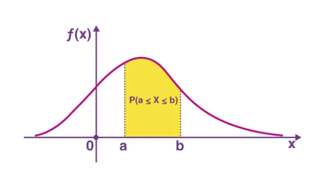
PDF. Source: Byjus
CDF: cumulative distribution function
The CDF returns the probability that a random variable X takes a value less than or equal to x.
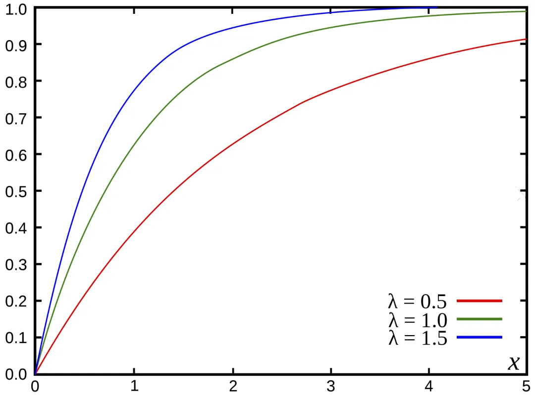
CDF (cumulative distribution function of the exponential distribution). Source: Wikipedia
3. Discrete distributions
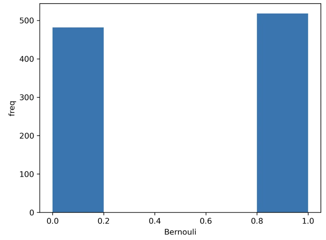
Bernoulli distribution
We have a single trial (one observation) with two possible outcomes, for example a coin toss. We have a true (1) result and a false (0) result. Assume heads corresponds to true (success). If the probability of heads is p, the complementary probability is 1-p.
import seaborn as sns from scipy.stats import bernoulli # Single observation # Generate data (1000 points, possible outs: 1 or 0, probability: 50% for each) data = bernoulli.rvs(size=1000,p=0.5) # Plot ax = sns.distplot(data_bern,kde=False,hist_kws={"linewidth": 10,'alpha':1}) ax.set(xlabel='Bernouli', ylabel='freq')