17 Common Machine Learning Algorithms

Overview

Different data types require different modeling approaches. In the fields of machine learning and artificial intelligence, the first consideration is how algorithms learn. There are several main learning paradigms. Classifying algorithms by learning paradigm helps when choosing models that best match the input data and the modeling task.

Learning Paradigms

1. Supervised learning

In supervised learning, input data are called training data and each training instance has an associated label or outcome, for example "spam" vs "not spam" in an email filter or the digits "1", "2", "3", "4" in handwritten digit recognition. Supervised learning builds a predictive model by comparing predictions to the actual labels in the training data and iteratively adjusting the model until a target accuracy is reached. Typical applications include classification and regression. Common algorithms include logistic regression and backpropagation neural networks.

2. Unsupervised learning

Unsupervised learning works with unlabeled data and attempts to infer intrinsic structure in the data. Common applications include association rule learning and clustering. Typical algorithms include the Apriori algorithm and k-means clustering.

3. Semi-supervised learning

Semi-supervised methods use datasets where some samples are labeled and others are not. These models can be used for prediction but usually first learn the data structure to organize unlabeled instances before applying supervised prediction. Typical applications include classification and regression; algorithms are often extensions of supervised methods that first model the unlabeled data and then refine predictions on labeled data. Examples include graph inference and Laplacian SVM.

4. Reinforcement learning

In reinforcement learning, inputs act as feedback to the model. Unlike supervised learning where labels serve only as checks for correctness, reinforcement learning provides rewards or penalties that the model uses to update policy immediately. Typical applications include dynamic systems and robotics control. Common algorithms include Q-learning and temporal-difference learning.

In enterprise data applications, supervised and unsupervised models are most common. In image recognition and related domains where large amounts of unlabeled data coexist with smaller labeled sets, semi-supervised learning is an active area. Reinforcement learning is more focused on control problems such as robotics and system control.

Algorithm Families by Similarity

Algorithms can also be grouped by functional or structural similarity, such as tree-based methods or neural networks. Some algorithms are hard to categorize uniquely. Algorithms within the same family can often address different problem types. The following sections classify commonly used algorithms by broadly understandable categories.

5. Regression algorithms

Regression algorithms measure error to explore relationships between variables and are a cornerstone of statistical machine learning. "Regression" can refer to a class of problems or to specific algorithms, which can confuse beginners. Common regression algorithms include ordinary least squares, logistic regression, stepwise regression, multivariate adaptive regression splines (MARS), and locally estimated scatterplot smoothing (LOESS).

6. Instance-based algorithms

Instance-based methods build decision models by retaining a set of sample instances and comparing new instances to these samples using similarity measures. These are also known as "memory-based" or "winner-take-all" learning. Common examples are k-nearest neighbors (KNN), learning vector quantization (LVQ), and self-organizing maps (SOM).

7. Regularization methods

Regularization methods extend other algorithms (often regression) by adjusting model complexity. Regularization typically rewards simpler models and penalizes complexity. Common techniques include ridge regression, least absolute shrinkage and selection operator (LASSO), and the elastic net.

8. Decision tree learning

Decision tree algorithms create tree-structured decision models based on data attributes and are used for classification and regression. Common methods include classification and regression trees (CART), ID3, C4.5, CHAID, decision stumps, random forest, MARS, and gradient boosting machines (GBM).

9. Bayesian methods

Bayesian algorithms are based on Bayes' theorem and are applied to classification and regression. Examples include naive Bayes, averaged one-dependence estimators (AODE), and Bayesian belief networks.

10. Kernel-based methods

Support vector machines (SVM) are the most well-known kernel-based techniques. Kernel methods map input data into higher-dimensional feature spaces where classification or regression tasks may be easier. Examples include support vector machines, radial basis function methods, and linear discriminant analysis (LDA).

11. Clustering algorithms

Like regression, clustering can refer to a problem type or a set of algorithms. Clustering algorithms aggregate input data by central points or hierarchical structure to reveal intrinsic groupings. Common methods include k-means and expectation-maximization (EM).

12. Association rule learning

Association rule learning discovers rules that best explain relationships among variables in large datasets. Typical algorithms include Apriori and Eclat.

13. Artificial neural networks

Artificial neural networks mimic biological neural systems and form a large family of pattern-matching algorithms for classification and regression. There are hundreds of variants; deep learning is a subset that will be discussed separately. Important network types include perceptrons, backpropagation networks, Hopfield networks, self-organizing maps (SOM), and LVQ.

14. Deep learning

Deep learning refers to developments in artificial neural networks, building much larger and more complex networks. Interest in deep learning has grown with increasing compute availability; after major investments in deep learning by companies such as Baidu, it gained additional attention in the Chinese market. Many deep learning approaches are semi-supervised and aim to handle large datasets with limited labels. Common models include restricted Boltzmann machines (RBM), deep belief networks (DBN), convolutional neural networks, and stacked autoencoders.

15. Dimensionality reduction

Dimensionality reduction methods analyze intrinsic data structure and aim to summarize or explain data with fewer variables. These unsupervised methods are used for visualization or to reduce complexity before supervised learning. Common techniques include principal component analysis (PCA), partial least squares (PLS), Sammon mapping, multidimensional scaling (MDS), and projection pursuit.

16. Ensemble methods

Ensemble algorithms train several relatively weak learning models independently on the same data and combine their results for overall prediction. Key challenges are which base learners to include and how to combine their outputs. Ensembles are powerful and widely used. Examples include boosting, bagging, AdaBoost, stacked generalization (blending), gradient boosting machines (GBM), and random forests.

Common Algorithm Advantages and Disadvantages

Naive Bayes

When feature vectors have varying lengths, they must be normalized to a common length. In text classification, for instance, a sentence can be represented as a vector with one dimension per vocabulary term and counts for each position.

The conditional probability for a class can be factorized under the naive Bayes independence assumption. If any conditional probability term is zero, the product can become zero. To avoid this, Laplace smoothing initializes counts (for binary classification add 1 to numerator and 2 to denominator; for k classes add k to denominator).

Advantages: Performs well on small datasets, suitable for multiclass tasks, and supports incremental training.

Disadvantages: Sensitive to how input data are represented.

Decision trees

A key step in decision trees is selecting an attribute for branching, which relies on information gain. Entropy is used to measure impurity, and information gain is the reduction in entropy after splitting. Evaluate all attributes and choose the one with the largest gain.

Advantages: Simple computation, strong interpretability, handles missing attribute values, and can work with irrelevant features.

Disadvantages: Prone to overfitting; ensembles such as random forests reduce overfitting.

Logistic regression

Logistic regression is a linear classifier used for classification. The logistic function and its derivative are used to model probabilities and train via maximum likelihood estimation. The loss is the negative log-likelihood and can be minimized with gradient descent.

Advantages: Easy to implement, low computational and storage cost at prediction time.

Disadvantages: Prone to underfitting; typically lower accuracy for complex problems. Standard logistic regression handles binary problems; softmax generalizes to multiclass. It assumes linear separability in the feature space without kernel extensions.

Linear regression

Linear regression is used for regression tasks. Parameters can be obtained by gradient descent optimizing the least squares loss, or directly via the normal equation. In locally weighted linear regression (LWLR), parameters are computed using a weighting matrix, making LWLR a nonparametric method since it requires evaluating training samples for each prediction.

Advantages: Simple to implement and compute.

Disadvantages: Cannot model nonlinear relationships without feature transformations.

K-Nearest Neighbors (KNN)

KNN classifies a test instance by:

1. computing distances between the test instance and all training samples (common metrics include Euclidean or Mahalanobis distance);
2. sorting these distances;
3. selecting the k closest samples;
4. voting among their labels to determine the predicted class.

Choosing k depends on the data. Larger k reduces noise sensitivity but blurs class boundaries; cross-validation is commonly used to select k. Noise and irrelevant features reduce KNN accuracy. As data size grows, KNN's error is bounded in relation to the Bayes error under certain conditions.

Note: Mahalanobis distance requires the sample mean vector and covariance matrix. Advantages include conceptual simplicity, mature theory, support for classification and regression, suitability for nonlinear problems, training time O(n), and robustness to outliers. Disadvantages include high computation and memory requirements and sensitivity to class imbalance.

Support Vector Machines (SVM)

Using libraries such as libsvm and tuning parameters is important. The SVM optimal hyperplane maximizes the geometric margin for all training samples. After derivations, SVM optimization can be expressed in primal form and then converted to a dual Lagrangian form. Solving for Lagrange multipliers α yields model parameters w and b. Kernel functions can replace the inner product in the prediction function, enabling nonlinear decision boundaries. Slack variables introduce a soft margin, which leads to an upper bound on α in the dual problem.

Advantages: Applicable to linear and nonlinear classification and regression, low generalization error, interpretable, and often computationally efficient.

Disadvantages: Sensitive to parameter and kernel choices and originally tailored for binary classification.

Boosting (AdaBoost)

AdaBoost trains multiple weak classifiers in sequence. Each weak learner is trained on weighted samples; misclassified examples receive increased weight for the next learner. Each weak classifier receives a weight α computed from its error rate ε. At prediction time, weighted votes from the weak classifiers are summed and the sign gives the final prediction.

Advantages: Low generalization error, relatively easy to implement, yields high accuracy with few tunable parameters.

Disadvantages: Sensitive to outliers.

Clustering

Clustering methods can be grouped by approach:

1. Partition-based clustering: k-means, k-medoids, CLARANS. k-means minimizes within-cluster squared error and is simple and scalable (complexity O(nkt)); however, it requires k in advance, is sensitive to initialization, and is not suitable for nonconvex clusters or clusters of very different sizes.
2. Hierarchical clustering: agglomerative methods like AGNES and divisive methods like DIANA.
3. Density-based clustering: DBSCAN, OPTICS, BIRCH (CF-tree), CURE.
4. Grid-based methods: STING, WaveCluster.
5. Model-based clustering: EM, SOM, COBWEB.

Recommender Systems

Recommender systems are commonly implemented via content-based methods and collaborative filtering.

Content-based: Treat ratings as a regression problem. Extract a feature vector for each item and learn a regression model for each user where the item features are inputs and the user's ratings are targets. Alternatively, infer item features from user preferences and optimize both user preferences and item features jointly.

Collaborative filtering: Can be viewed as a classification or matrix factorization problem. CF leverages similarities in users' preferences without relying on item features. Matrix factorization via singular value decomposition (SVD) decomposes the data matrix into three matrices. The diagonal matrix contains singular values sorted in descending order; low-rank approximations using the largest singular values can reconstruct the original matrix approximately and reduce dimensionality. For example, with m items and n users, rows of the U matrix represent item attributes in a reduced k-dimensional space. A new user's vector can be projected and compared to existing user vectors to find similar users for recommendations.

Probabilistic Topic Models

pLSA evolved from latent semantic analysis (LSA), where early LSA implementations relied on SVD. pLSA uses a probabilistic model; the model diagram shows latent topics conditioning words and documents. Latent Dirichlet allocation (LDA) differs by assuming priors, commonly Dirichlet priors, because conjugate priors simplify inference by preserving posterior form.

Gradient Boosting Decision Trees (GBDT)

GBDT, also called MART (Multiple Additive Regression Tree), is an iterative decision tree ensemble where the final output is the sum of many regression trees. Each tree fits the residuals of the ensemble so far. Regularization and boosting reduce overfitting. GBDT is recognized for strong generalization performance and has been widely used in learning-to-rank and other tasks.

Regularization

Regularization helps in several ways:

1. Numerical stability in optimization;
2. Stability when the number of features is large;
3. Controls model complexity and smoothness—simpler, smoother objective functions generalize better;
4. Reduces the parameter space and hence model complexity;
5. Smaller coefficients correspond to simpler models and often better generalization;
6. Can be interpreted as placing a Gaussian prior on weights.

Anomaly Detection

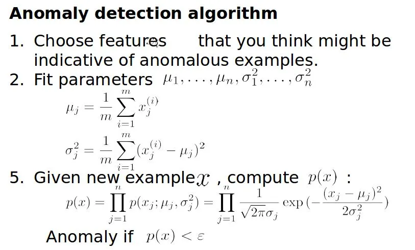
Anomaly detection often estimates the sample density function; new samples with density below a threshold are flagged as anomalies. Multivariate Gaussian distributions are commonly used. When features do not appear Gaussian, transformations like log or power transforms can help. The threshold ε can be chosen by cross-validation. Anomaly detection combines unsupervised density estimation for p(x) with supervised selection of ε because labeled anomalies are scarce and insufficient for conventional supervised training.

Expectation-Maximization (EM)

When sample generation involves latent variables that are not observed, maximum likelihood estimation becomes difficult. The EM algorithm iteratively estimates parameters in two steps:

E-step: Using current parameters, compute the conditional distribution of latent variables.

M-step: Maximize the expected complete-data log-likelihood under the latent variable distribution computed in the E-step. Repeat until convergence. EM is widely used for Gaussian mixture models (GMM), where each sample can be generated by one of k Gaussians with different mixing weights. EM alternates between computing posterior probabilities for each component (E-step) and updating component weights, means, and covariances (M-step).

Association Rule Mining: Apriori and FP-Growth

Apriori finds frequent itemsets using the property that a superset of an infrequent set cannot be frequent. Apriori scans the transaction table multiple times, pruning non-frequent candidates at each pass and generating larger candidate sets iteratively.

FP-Growth is a more efficient method that requires only two scans of the transaction database. The first scan counts item frequencies and prunes infrequent items; the second scan builds an FP-tree. Frequent patterns are mined by recursively extracting conditional pattern bases and building smaller FP-trees for each item.

Examples and diagrams in the original content illustrate these processes and the FP-tree construction.

Summary

This document summarized 17 common machine learning algorithm families, their typical applications, and key advantages and limitations. The chosen algorithm depends on the data characteristics, task requirements, and computational constraints.