ALLPCB


Researchers introduced the concept of convolutional neural networks (CNNs) while studying image processing algorithms. Traditional fully connected networks act as a black box: they take all inputs, pass each value through a dense network, and then produce a one-hot output. That approach can work with a small number of inputs.
For a 1024x768 image, the input is 3 x 1024 x 768 = 2,359,296 numbers (RGB per pixel). A dense multilayer neural network with input vectors of that size would require at least 2,359,296 weights per neuron in the first layer — about 2 MB of weights for each neuron in the first layer. For typical processors and RAM available before the 2000s, that was impractical.
This motivated researchers to look for a better approach. The first and most important task in any image processing or recognition pipeline is often detecting edges and textures. Object recognition and higher-level processing follow. It is clear that detecting textures and edges does not require the entire image: one only needs to examine the pixels around a given pixel to identify an edge or texture.
Furthermore, the algorithm used to detect an edge or texture should be the same across the image. We cannot use different algorithms for the center, corners, or sides of the image. The concept of detecting edges or texture must be uniform, so we do not need to learn a separate set of parameters for each pixel.
This insight led to convolutional neural networks. The first layer of the network is composed of neurons that scan small patches of the image, processing a few pixels at a time. Common patch sizes are 9, 16, or 25 pixels arranged as small squares.
CNNs greatly reduce computation. Small filters or kernels slide across the image, processing a small patch at each step. Because the processing required across the image is very similar, this approach is highly efficient.
Although CNNs were introduced for image processing, over the years they have been applied in many other domains.
Example
Now that we understand the basic concept of CNNs, let's see how they work on digits and how CNNs solve the edge detection problem. Edge detection is a core task in many image-processing problems. The example below shows how a convolutional filter highlights edges.
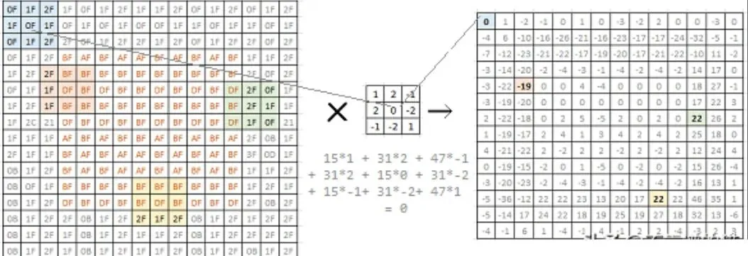
The left image is a 16x16 grayscale bitmap. Each matrix value represents pixel brightness. A simple square appears in the middle. Convolving this image with a 2x2 filter (center) yields a 14x14 matrix (right).
The chosen filter can emphasize edges. In the right matrix, values corresponding to edges in the original image are high (positive or negative). This is a simple edge-detection filter. Researchers have identified many different filters to pick up and emphasize various image aspects. In typical CNN model development, the network learns these filters itself.
Important Concepts
Below are some key concepts to understand before working further with CNNs.
Padding
A common issue with convolutional filters is that each step reduces the output size, which effectively loses “information.” If the input is N x N and the filter is F x F, the output becomes (N - F + 1) x (N - F + 1) because pixels at the edges are covered fewer times than pixels near the center.
Padding the image on all sides by (F - 1) / 2 pixels preserves the original N x N size.
There are two main types of convolution: valid convolution and same convolution. Valid means no padding, so each convolution reduces the size. Same convolution uses padding to preserve the matrix size.
In computer vision, F is usually odd. An odd F helps maintain image symmetry and allows a center pixel, which is useful for applying uniform biases. Common filter sizes are 3x3, 5x5, and 7x7. There are also 1x1 filters.
Stride
The convolutions discussed above scan pixels sequentially. We can also use strides, which skip s pixels when the filter moves across the image.
If the input is n x n and the filter is f x f, using stride s and padding p produces an output of ((n + 2p - f) / s + 1) x ((n + 2p - f) / s + 1).
Convolution vs Cross-correlation
Cross-correlation is essentially convolution without flipping the filter across the main diagonal. Flipping introduces an extra correlation, but in image processing we usually do not flip the filter.
Convolution on RGB Images
For an n x n x 3 image and an f x f x 3 filter, both image and filter have height, width, and channels. The number of channels in the image must match the number of channels in the filter. The output has width and height (n - f + 1) and a single channel per filter.
Multiple Filters
A 3-channel image convolved with one 3-channel filter yields a single-channel output. However, we can use multiple filters — each filter produces a separate output layer. The number of filters equals the number of output channels or feature maps.
Starting from a 3-channel image, we can end up with many output channels. Each output channel represents a particular feature of the image captured by the corresponding filter. In deep networks, we also add a bias and a nonlinear activation function such as ReLU.
Pooling Layers
Pooling combines values into a single value. There are average pooling, max pooling, min pooling, and others. Applying f x f pooling to an n x n input results in (n / f) x (n / f) output. Pooling layers have no parameters to learn.
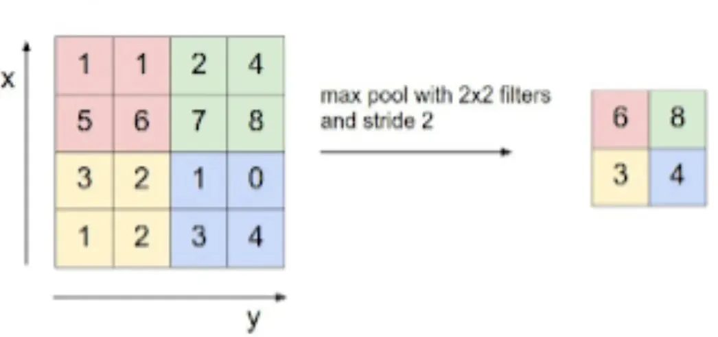
Max pooling
CNN Architecture
Typical small to medium CNN models follow a few general principles.
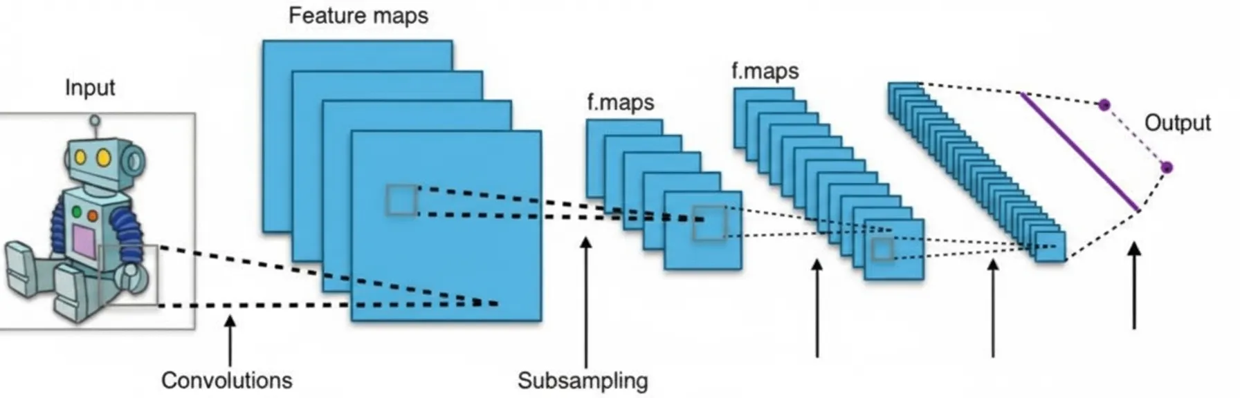
Common design patterns:
- Alternate convolutional and pooling layers
- Gradually reduce spatial dimensions while increasing the number of feature maps
- Toward the end, flatten followed by fully connected layers
- Use ReLU for hidden layers, and softmax for the final layer
For large and very large networks, architectures become more complex. Researchers have proposed many specific architectures for large-scale tasks, such as ImageNet, GoogLeNet, and VGGNet.
Python Implementation
When implementing a CNN, start with data analysis and cleaning, then choose a network model. Define the architecture — number of layers, layer sizes, and connectivity — and allow the network to learn the parameters. Adjust hyperparameters to get a model that meets the requirements.
Below is a simple example showing how a convolutional network works.
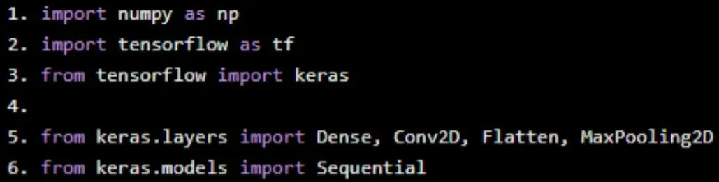
Import modules
import numpy as np
import tensorflow as tf
from tensorflow import keras
from keras.layers import Dense, Conv2D, Flatten, MaxPooling2D
from keras.models import Sequential
Get data
Next, obtain the data. We use the MNIST dataset built into Keras. In practice, this requires more preprocessing.
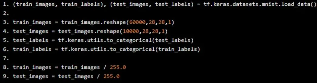
Load training and test data. Reshape the data to fit the convolutional network: reshape into 4D arrays with 60,000 records of size 28x28x1 for training. This makes building convolutional layers in Keras straightforward.
(train_images, train_labels), (test_images, test_labels) = tf.keras.datasets.mnist.load_data()
train_images = train_images.reshape(60000,28,28,1)
test_images = test_images.reshape(10000,28,28,1)
test_labels = tf.keras.utils.to_categorical(test_labels)
train_labels = tf.keras.utils.to_categorical(train_labels)
train_images = train_images / 255.0
test_images = test_images / 255.0
Build the model
The Keras library provides an API for building models. Create a Sequential model instance and add layers. The first layer is a convolutional layer handling 28x28 input images. Define kernel size 3 and create 32 such kernels — producing 32 output feature maps of size 26x26 (28 - 3 + 1 = 26).
model = Sequential()
model.add(Conv2D(32, kernel_size=3, activation='relu', input_shape=(28,28,1)))
model.add(MaxPooling2D(pool_size=(3, 3)))
model.add(Conv2D(24, kernel_size=3, activation='relu'))
model.add(MaxPooling2D(pool_size=(2, 2)))
model.add(Flatten())
model.add(Dense(10, activation='softmax'))
model.compile(optimizer='adam', loss='categorical_crossentropy', metrics=['accuracy'])
Train the model
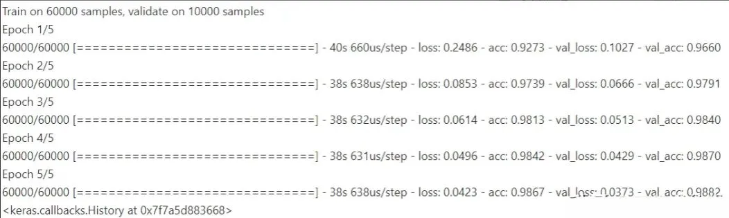
Finally, train the model with available data. Five epochs are usually sufficient to get a reasonably accurate model for this simple example.
model.fit(train_images, train_labels, validation_data=(test_images, test_labels), epochs=5)
Conclusion
The example model above only needs 9*32 + 9*24 = 504 values to learn. A fully connected network would require 784 weights per neuron in the first layer. CNNs therefore greatly reduce computation and also reduce the risk of overfitting. The approach uses known priors about images and then trains the model to discover the rest. A black-box fully connected or randomly sparse network would not achieve this accuracy at the same computational cost.