ALLPCB


Overview
A Gaussian filter is a linear filter that effectively suppresses noise and smooths images. Its principle is similar to the mean filter: the output for a pixel is computed from the values inside the filter window. The difference is that a mean filter uses equal coefficients, while a Gaussian filter uses coefficients that decrease with distance from the kernel center. As a result, a Gaussian filter produces less blurring than a mean filter for the same window size.
What is a Gaussian filter
The name refers to the Gaussian (normal) distribution. The two-dimensional Gaussian function is used to form the kernel by discretizing the continuous function and using the sampled values as kernel coefficients.
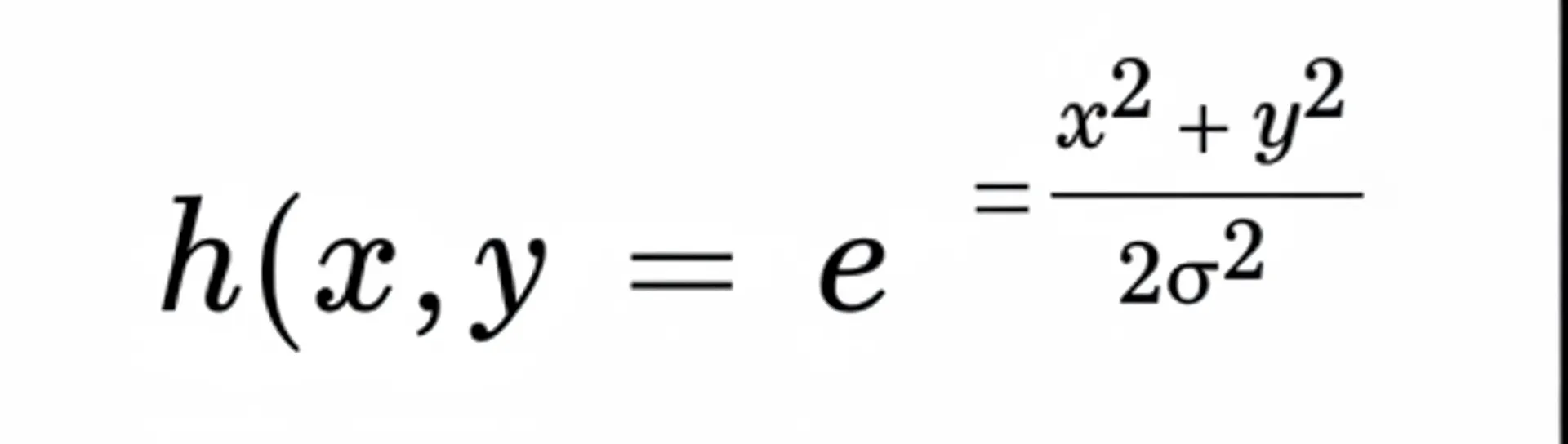
Treat (x, y) as integer coordinates in image processing and sigma as the standard deviation. To generate a kernel, sample the Gaussian function with the kernel center as the origin. For example, for a 3x3 kernel, use the center as (0, 0) and sample coordinates as shown below.
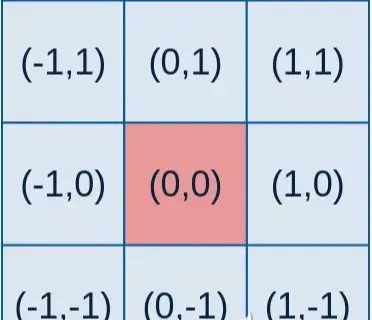
Substitute each coordinate into the Gaussian function to obtain the corresponding kernel coefficient. For a window size of (2k+1)x(2k+1), each element is computed by the Gaussian formula shown below.
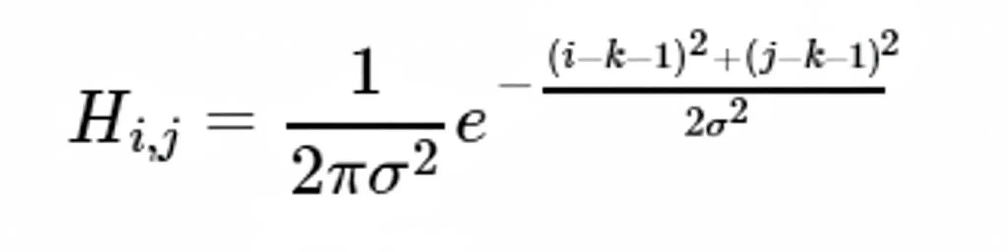
Computed kernels can be represented either as floating-point values or as integers. Floating-point kernels are the direct sampled values. Integer kernels require normalization and rounding. One common integer approach is to normalize the top-left coefficient to 1 and scale all elements accordingly; then apply an overall factor equal to the reciprocal of the sum of integer coefficients during convolution.
Generating the Gaussian kernel
Knowing the generation principle, implementing the kernel is straightforward. Example code (integer-normalization approach):
void generateGaussianTemplate(double window[][11], int ksize, double sigma)
{
    static const double pi = 3.1415926;
    int center = ksize / 2; // Center position of the kernel, i.e. the origin
    double x2, y2;
    for (int i = 0; i < ksize; i++)
    {
        x2 = pow(i - center, 2);
        for (int j = 0; j < ksize; j++)
        {
            y2 = pow(j - center, 2);
            double g = exp(-(x2 + y2) / (2 * sigma * sigma));
            g /= 2 * pi * sigma;
            window[i][j] = g;
        }
    }
    double k = 1 / window[0][0]; // Normalize so the top-left coefficient becomes 1
    for (int i = 0; i < ksize; i++)
    {
        for (int j = 0; j < ksize; j++)
        {
            window[i][j] *= k;
        }
    }
}
This implementation requires a 2D array to store coefficients (here the maximum kernel size is assumed to be 11). The second parameter is the kernel size and the third is the Gaussian standard deviation sigma. The algorithm computes the center index, samples the Gaussian at each kernel coordinate, and then performs normalization by scaling with the reciprocal of the top-left value. Rounding the scaled values yields an integer kernel.
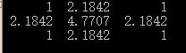
Below is an example set of generated kernels for 3x3 with sigma values around 0.8.
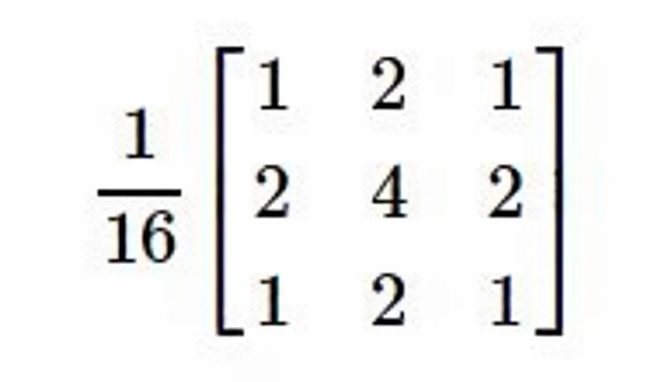
For a floating-point kernel, skip the integer normalization and divide each sampled coefficient by the sum of all coefficients. Example code:
void generateGaussianTemplate(double window[][11], int ksize, double sigma)
{
    static const double pi = 3.1415926;
    int center = ksize / 2; // Center position of the kernel, i.e. the origin
    double x2, y2;
    double sum = 0;
    for (int i = 0; i < ksize; i++)
    {
        x2 = pow(i - center, 2);
        for (int j = 0; j < ksize; j++)
        {
            y2 = pow(j - center, 2);
            double g = exp(-(x2 + y2) / (2 * sigma * sigma));
            g /= 2 * pi * sigma;
            sum += g;
            window[i][j] = g;
        }
    }
    for (int i = 0; i < ksize; i++)
    {
        for (int j = 0; j < ksize; j++)
        {
            window[i][j] /= sum;
        }
    }
}
Meaning and selection of sigma
The most important parameter for a Gaussian kernel is the standard deviation sigma. Sigma represents dispersion: a small sigma produces a kernel with a large central coefficient and small neighbors, causing limited smoothing; a large sigma flattens the kernel so coefficients are more similar, producing stronger smoothing similar to a mean filter.
In the one-dimensional Gaussian probability density plot, the horizontal axis is the variable x and the vertical axis is the density f(x). The total area under the curve is 1. Sigma controls the curve width: larger sigma yields a wider, lower peak; smaller sigma yields a narrower, sharper peak. Therefore:
- Large sigma: distribution is spread out, kernel coefficients are similar, resulting in stronger smoothing.
- Small sigma: distribution is concentrated, central coefficient dominates, producing a local weighted average close to a point operation.
OpenCV-based implementation
Once the kernel is generated, applying it via convolution is straightforward. Example implementation using OpenCV data structures:
void GaussianFilter(const Mat &src, Mat &dst, int ksize, double sigma)
{
    CV_Assert(src.channels() == 1 || src.channels() == 3); // Only process single-channel or three-channel images
    const static double pi = 3.1415926;
    // Generate Gaussian kernel based on window size and sigma
    // Allocate a 2D array to store the kernel matrix
    double **templateMatrix = new double*[ksize];
    for (int i = 0; i < ksize; i++)
        templateMatrix[i] = new double[ksize];
    int origin = ksize / 2; // Use kernel center as origin
    double x2, y2;
    double sum = 0;
    for (int i = 0; i < ksize; i++)
    {
        x2 = pow(i - origin, 2);
        for (int j = 0; j < ksize; j++)
        {
            y2 = pow(j - origin, 2);
            // The constant factor before the Gaussian can be omitted and will be removed in normalization
            double g = exp(-(x2 + y2) / (2 * sigma * sigma));
            sum += g;
            templateMatrix[i][j] = g;
        }
    }
    for (int i = 0; i < ksize; i++)
    {
        for (int j = 0; j < ksize; j++)
        {
            templateMatrix[i][j] /= sum;
            cout << templateMatrix[i][j] << " ";
        }
        cout << endl;
    }
    // Apply the kernel to the image
    int border = ksize / 2;
    copyMakeBorder(src, dst, border, border, border, border, BorderTypes::BORDER_REFLECT);
    int channels = dst.channels();
    int rows = dst.rows - border;
    int cols = dst.cols - border;
    for (int i = border; i < rows; i++)
    {
        for (int j = border; j < cols; j++)
        {
            double sum[3] = { 0 };
            for (int a = -border; a <= border; a++)
            {
                for (int b = -border; b <= border; b++)
                {
                    if (channels == 1)
                    {
                        sum[0] += templateMatrix[border + a][border + b] * dst.at<uchar>(i + a, j + b);
                    }
                    else if (channels == 3)
                    {
                        Vec3b rgb = dst.at<Vec3b>(i + a, j + b);
                        auto k = templateMatrix[border + a][border + b];
                        sum[0] += k * rgb[0];
                        sum[1] += k * rgb[1];
                        sum[2] += k * rgb[2];
                    }
                }
            }
            for (int k = 0; k < channels; k++)
            {
                if (sum[k] < 0)
                    sum[k] = 0;
                else if (sum[k] > 255)
                    sum[k] = 255;
            }
            if (channels == 1)
                dst.at<uchar>(i, j) = static_cast<uchar>(sum[0]);
            else if (channels == 3)
            {
                Vec3b rgb = { static_cast<uchar>(sum[0]), static_cast<uchar>(sum[1]), static_cast<uchar>(sum[2]) };
                dst.at<Vec3b>(i, j) = rgb;
            }
        }
    }
    // Release the kernel array
    for (int i = 0; i < ksize; i++)
        delete[] templateMatrix[i];
    delete[] templateMatrix;
}
This direct convolution has computational cost proportional to m×n×ksize^2, where m and n are image dimensions and ksize is the kernel size. Complexity per pixel is O(ksize^2). For large kernels this becomes inefficient, but the Gaussian function is separable, which enables a faster approach.
Separable implementation
Because the 2D Gaussian is separable, you can perform two 1D convolutions: first convolve rows with a 1D Gaussian, then convolve columns with the same 1D kernel. This reduces computation and makes the cost grow linearly with kernel size.
// Separable implementation
void separateGaussianFilter(const Mat &src, Mat &dst, int ksize, double sigma)
{
    CV_Assert(src.channels() == 1 || src.channels() == 3); // Only process single-channel or three-channel images
    // Generate 1D Gaussian kernel
    double *matrix = new double[ksize];
    double sum = 0;
    int origin = ksize / 2;
    for (int i = 0; i < ksize; i++)
    {
        // The constant factor before the Gaussian can be omitted and will be removed in normalization
        double g = exp(-(i - origin) * (i - origin) / (2 * sigma * sigma));
        sum += g;
        matrix[i] = g;
    }
    // Normalize
    for (int i = 0; i < ksize; i++)
        matrix[i] /= sum;
    // Apply the kernel to the image
    int border = ksize / 2;
    copyMakeBorder(src, dst, border, border, border, border, BorderTypes::BORDER_REFLECT);
    int channels = dst.channels();
    int rows = dst.rows - border;
    int cols = dst.cols - border;
    // Horizontal pass
    for (int i = border; i < rows; i++)
    {
        for (int j = border; j < cols; j++)
        {
            double sum[3] = { 0 };
            for (int k = -border; k <= border; k++)
            {
                if (channels == 1)
                {
                    sum[0] += matrix[border + k] * dst.at<uchar>(i, j + k); // Row fixed, column varies; horizontal convolution
                }
                else if (channels == 3)
                {
                    Vec3b rgb = dst.at<Vec3b>(i, j + k);
                    sum[0] += matrix[border + k] * rgb[0];
                    sum[1] += matrix[border + k] * rgb[1];
                    sum[2] += matrix[border + k] * rgb[2];
                }
            }
            for (int k = 0; k < channels; k++)
            {
                if (sum[k] < 0)
                    sum[k] = 0;
                else if (sum[k] > 255)
                    sum[k] = 255;
            }
            if (channels == 1)
                dst.at<uchar>(i, j) = static_cast<uchar>(sum[0]);
            else if (channels == 3)
            {
                Vec3b rgb = { static_cast<uchar>(sum[0]), static_cast<uchar>(sum[1]), static_cast<uchar>(sum[2]) };
                dst.at<Vec3b>(i, j) = rgb;
            }
        }
    }
    // Vertical pass
    for (int i = border; i < rows; i++)
    {
        for (int j = border; j < cols; j++)
        {
            double sum[3] = { 0 };
            for (int k = -border; k <= border; k++)
            {
                if (channels == 1)
                {
                    sum[0] += matrix[border + k] * dst.at<uchar>(i + k, j); // Column fixed, row varies; vertical convolution
                }
                else if (channels == 3)
                {
                    Vec3b rgb = dst.at<Vec3b>(i + k, j);
                    sum[0] += matrix[border + k] * rgb[0];
                    sum[1] += matrix[border + k] * rgb[1];
                    sum[2] += matrix[border + k] * rgb[2];
                }
            }
            for (int k = 0; k < channels; k++)
            {
                if (sum[k] < 0)
                    sum[k] = 0;
                else if (sum[k] > 255)
                    sum[k] = 255;
            }
            if (channels == 1)
                dst.at<uchar>(i, j) = static_cast<uchar>(sum[0]);
            else if (channels == 3)
            {
                Vec3b rgb = { static_cast<uchar>(sum[0]), static_cast<uchar>(sum[1]), static_cast<uchar>(sum[2]) };
                dst.at<Vec3b>(i, j) = rgb;
            }
        }
    }
    delete[] matrix;
}
By separating the 2D convolution into two 1D convolutions, the algorithm's computational cost grows linearly with kernel size rather than quadratically.
OpenCV also provides a built-in GaussianBlur function with the signature:
CV_EXPORTS_W void GaussianBlur( InputArray src, OutputArray dst, Size ksize,
                                  double sigmaX, double sigmaY = 0,
                                  int borderType = BORDER_DEFAULT );
In OpenCV, sigmaX and sigmaY allow different standard deviations for the x and y directions. In the examples above, the same sigma was used for both directions.
Summary
A Gaussian filter is a linear smoothing filter whose kernel is derived from sampling a two-dimensional Gaussian function. Because the kernel values are largest at the center and taper toward the edges, Gaussian filtering preserves image structure better than a simple mean filter. The key parameter is the Gaussian standard deviation sigma: larger sigma increases smoothing and widens the filter's effective frequency band, while smaller sigma reduces smoothing and keeps details sharper. Adjusting sigma balances noise suppression and image blurring.