ALLPCB


Introduction
In engineering practice, visual-inertial odometry (VIO), which fuses camera and inertial measurement unit (IMU) data, is generally preferred over pure visual odometry (VO) for motion estimation. The advantage of VIO stems from the complementary characteristics of cameras and IMUs.
Sensor Complementarity
Cameras perform well in most texture-rich scenes, but they struggle in feature-poor environments such as glass surfaces or blank walls. A key benefit of cameras is that their estimates do not drift: if a camera is fixed, the estimated pose remains fixed.
IMUs have their own drawbacks. Over long durations, IMU integration accumulates large errors. However, over short intervals IMU relative displacement estimates can be highly accurate, so fusing IMU data improves localization when visual sensing fails. IMUs measure angular velocity and linear acceleration, but these signals include biases and noise that produce drift when integrated. If an IMU is stationary, integration drift still causes the integrated pose to wander. Conversely, for short, rapid motions where a camera may blur or have insufficient inter-frame overlap for feature matching, the IMU provides useful complementary information. For these reasons, many SLAM algorithms fuse camera and IMU data for pose estimation.
Preintegration: Concept and Motivation
One concept commonly associated with VIO is preintegration. IMUs typically sample at high rates (100 Hz to 1000 Hz), producing large amounts of data. In optimization-based back ends, it is impractical to include every IMU sample as a state variable. A common approach is to extract states at coarser intervals, for example every second. Given the state (position, velocity, attitude) at time i, and all IMU measurements between times i and j, one can integrate the IMU kinematics to obtain the state at time j.
However, during iterative back-end optimization, if the state at time i is updated, all intermediate integrations up to time j would need to be recomputed, which becomes expensive when hundreds of IMU samples are involved. Preintegration attempts to replace many integrations with a single preintegrated measurement, dramatically reducing computation by summarizing the effect of the high-frequency IMU measurements between two states into one set of preintegrated quantities.
Preintegration Formulation
The preintegrated quantities depend only on IMU measurements; they are obtained by integrating the IMU data over the interval. Expressing the continuous integration model in a discrete preintegration form allows using one preintegrated measurement in the optimization instead of many raw samples.
Measured IMU signals are not the objective physical quantities but are corrupted by sensor errors, namely biases and noise. In notation, a and g denote accelerometer and gyroscope measurements. Superscripts w and b denote the world frame and the IMU body frame respectively. Many subscripts appear in the detailed formulas and can be confusing.
The time derivatives of position, velocity, and attitude (position, velocity, quaternion, or PVQ) can be written in a standard kinematic form. The first two equations are straightforward integrals relating the three motion quantities. The third equation describes the quaternion derivative; a short derivation of that quaternion relation is often provided for clarity.
Discrete Preintegration and Error Representation
Preintegration is typically implemented in discrete form. The preintegrated quantities summarize the displacement, velocity change, and relative rotation over the interval. Measurement errors for displacement, velocity, and biases are expressed as differences between measured and estimated values. Rotational errors are represented using quaternion error models.
Transforming the integration model into a preintegration model reduces computation, but it introduces a question of uncertainty: when many noisy IMU samples are collapsed into one preintegrated result, what is the covariance of that preintegrated value? Prior to preintegration, the noise variance of each IMU sample is known from calibration, but the variance of the integrated preintegrated quantities must be derived by propagating IMU noise through the integration model. This requires a linear propagation relationship between the IMU noise and the preintegrated quantities.
Covariance Propagation
Assuming a linearized error propagation between adjacent timesteps, the error at the next timestep is the result of propagating the current error and adding the contribution from current measurement noise. The covariance matrix of the preintegrated quantities can then be computed by recursive propagation. The detailed derivation uses Lie group and Lie algebra tools; the resulting expressions match those used in common open-source VIO implementations such as VINS-MONO.
Role of Preintegration in VIO Systems
In open-source VIO frameworks, IMU preintegration is part of the front end and is computed immediately after IMU data collection. A complete VIO system also includes initialization (aligning IMU and camera data) and the back-end optimization. The back end builds the overall objective function and typically uses a sliding window strategy to limit the number of states and control computational cost. Preintegration reduces the number of variables and the computation required during each optimization iteration.
Summary
Preintegration provides an efficient way to incorporate high-rate IMU data into optimization-based VIO by summarizing many samples into a single set of measurements and propagated covariances. This approach leverages the complementary strengths of cameras and IMUs to improve motion estimation in conditions where either sensor alone would be insufficient.