ALLPCB


Overview
Augmented reality evolved from virtual reality, so AR hardware inherits many structural similarities with VR systems. Like most VR systems, a graphics processor is essential for AR. AR systems also include human-computer interaction devices such as data gloves, 6D mice, eye trackers, force-feedback devices, and speech recognition and synthesis systems, each available in many variants with different performance characteristics.
Hardware trackers that obtain the tracked object's position and orientation are commonly used in AR systems. These hardware trackers include electromechanical trackers, electromagnetic trackers, ultrasonic trackers, optical trackers, and inertial trackers. Each uses different implementation methods, with distinct advantages and limitations, and all have application examples in current AR systems.
1. Electromechanical tracker
Electromechanical trackers are absolute-position sensors, typically built from a compact mechanical arm with one end fixed to a reference base and the other attached to the object being measured. Potentiometers or optical encoders are used as joint sensors to measure joint rotation. Using the measured relative joint angles and the arm lengths between sensors, the system computes a six-degree-of-freedom pose. These trackers tend to be reliable, have few interference sources, and exhibit low latency. Their drawbacks include sensitivity of measurement accuracy to environmental temperature changes, limited resolution of joint sensors, and restricted working range. They are advantageous in applications where user workspace is not a primary concern, such as surgical training.
2. Electromagnetic tracker
Electromagnetic trackers are widely used attitude trackers. They use a three-axis coil to emit a low-frequency magnetic field and a three-axis magnetic receiver mounted on the tracked object to sense the field. The coupling relationship between the emitted magnetic field and the induced signals is used to determine the spatial pose of the tracked object. Depending on the excitation source, electromagnetic trackers are classified as AC electromagnetic trackers and DC electromagnetic trackers.
AC electromagnetic trackers use bipolar magnetic sources produced by three orthogonal alternating currents, and the receiver consists of three sets of coils that measure each excitation source. The receiver senses the excitation fields and calculates the receiver?s pose relative to the source based on electromagnetic energy transfer. Considering computation, response time, and noise, excitation frequencies are typically 30–120 Hz. To ensure adequate signal-to-noise ratio in various environments, a 7–14 kHz carrier is often used to modulate the excitation waveform. DC electromagnetic trackers have transmitters composed of three orthogonally wound coils on a cube core. DC current is applied sequentially to the transmitter coils, producing pulse-modulated DC magnetic fields. Receivers are also three orthogonally wound coil sets; periodic changes in the DC field induce alternating currents in the receiver coils, with amplitudes proportional to the resolvable components of the local DC magnetic field. Each measurement cycle yields nine data values representing the magnitudes induced in the three receiver coil sets, and the electronics apply algorithms to determine the receiver?s position and orientation relative to the transmitter.
AC electromagnetic receivers are usually compact and suitable for mounting on head-mounted displays, but a major drawback is susceptibility to environmental electromagnetic interference. AC excitation fields are especially sensitive to nearby conductive materials, particularly ferromagnetic materials. AC rotating magnetic fields induce eddy currents in ferromagnetic materials, generating secondary AC fields that distort the original field pattern and cause significant measurement errors.
The main advantage of DC electromagnetic trackers is that eddy currents are produced only at the start of a measurement cycle. Once the magnetic field reaches steady state, eddy currents cease. Waiting for eddy currents to decay before measurement reduces eddy-current-related distortion and measurement errors.
3. Ultrasonic tracker
Ultrasonic tracking uses differences in arrival time, phase, or sound pressure from multiple sources to determine position. Two common approaches are pulse time-of-flight (time-of-flight, TOF) measurement and continuous-wave phase-coherent measurement. TOF measures the propagation time of a pulse between transmitter and receiver under known temperature conditions to determine distance; most ultrasonic trackers use this method. The data refresh rate is limited by factors including the speed of sound (~340 m/s). Valid measurements are obtained only when the wavefront reaches the sensor, and transmitters must emit millisecond-scale pulses and wait for them to dissipate before starting new measurements. Because each transmitter-receiver pair requires a separate pulse sequence, total measurement time equals single-pair flight time multiplied by the number of pairs. Accuracy depends on detecting the precise arrival time of the emitted pulse; ambient sounds, airflow, and sensor latching can degrade measurement accuracy.
Continuous-wave phase-coherent measurement compares the phase between a reference signal and the received signal to determine distance. This approach offers higher accuracy and higher data refresh rates and can use multiple filtering passes to mitigate environmental interference without compromising precision or response time.
Compared with electromagnetic trackers, ultrasonic trackers are immune to external magnetic fields and ferromagnetic materials, and they can offer larger measurement ranges. TOF-based trackers are vulnerable to spurious acoustic pulses but provide good accuracy and response in short ranges; however, accuracy and refresh rate typically decline with increased distance. Trackers based on continuous-wave coherent measurement provide higher refresh rates, improving precision, responsiveness, measurement range, and robustness, and are less affected by spurious pulses. Both methods can suffer errors from airflow or sensor latching, but appropriate modulation can improve environmental robustness and enable acoustic trackers with high accuracy, high refresh rate, and low latency.
Historically, in 1966 Roberts at MIT Lincoln Laboratory developed an ultrasonic displacement tracker called the Lincoln Wand. That eye tracker used TOF with four transmitters and one receiver and achieved about 5 mm accuracy and resolution. Logitech developed another TOF-based ultrasonic tracking system called RedBaron, which also achieved accuracy on the order of a few millimeters.
4. Optical tracker
Optical trackers, or visual trackers, use ambient or controlled light and the projections of that light on an image plane at different times or positions to compute the tracked object?s pose. When a controlled illumination source is used, infrared light is commonly chosen to avoid disturbing the user.
From a structural viewpoint, optical trackers are classified as outside-in (OI) and inside-out (IO). In an outside-in setup, sensors are fixed and emitters are mounted on the tracked object, meaning the sensors look inward at distant moving targets; such systems typically require expensive, high-resolution sensors. In an inside-out setup, emitters are fixed and sensors are mounted on the moving object, so the sensors look outward from the moving device. Using multiple emitters within the workspace can increase precision and extend the working range.
Inside-out optical trackers offer good temporal response, high data refresh rates, broad applicability, and low phase lag, making them well suited for real-time applications. Optical systems are, however, vulnerable to false light, surface blur, and occlusion. Using short-focus lenses to obtain sufficient working range can reduce measurement precision. Multi-emitter architectures can mitigate some issues but add complexity and cost. Therefore, optical trackers must balance accuracy, measurement range, and price, and they require an unobstructed optical path for reliable operation.
5. Inertial tracker
Inertial trackers use gyroscopes to track orientation and measure angular changes for three rotational degrees of freedom, and accelerometers to measure translational motion for three linear degrees of freedom. This approach was traditionally used in aircraft and missile navigation and tended to be bulky. As gyroscopes and accelerometers have been miniaturized, inertial tracking has become increasingly viable for civilian applications. The primary advantage is that inertial trackers do not require external transmitters. Traditional gyroscope technologies, however, often struggle to meet precision requirements: measurement errors accumulate over time as angular drift, and temperature-dependent drift is significant, necessitating temperature compensation. New piezoelectric solid-state gyroscopes have substantially improved performance in these areas.