ALLPCB


Consider a radiated emissions (RE102) limit chart from the Chinese military standard GJB151B. The vertical axis, representing field strength limits, is logarithmic. Let's perform a simple calculation to understand the range of this axis. It spans from 0 dBuV/m to 100 dBuV/m. In linear terms, 0 dBuV/m is equal to 1 uV/m, while 100 dBuV/m is equal to 100,000 uV/m. This represents a dynamic range of 100,000:1.
If we were to plot this on a linear scale with, for example, 10 grid divisions, each division would represent 10,000 uV/m. This value corresponds to 80 dBuV/m. Consequently, any value below 80 dBuV/m would be compressed into the first grid division, making smaller values impossible to distinguish. The resulting graph would be distorted and impractical.
Electromagnetic compatibility (EMC) testing often deals with a very wide range of field strengths. Using a linear scale makes it impossible to effectively visualize smaller values on a graph. By introducing the decibel (dB), we compress the numerical range logarithmically. This ensures that each tenfold increase in value occupies the same amount of space on the axis, allowing a single graph to clearly display values from very small to very large.
dB vs. dBuV: A Key Distinction
Engineers working in EMC know that power calculations use a factor of 10 (10log), while voltage calculations use a factor of 20 (20log). The formulas are available in standard reference materials. Here, we want to emphasize the distinction between dB and dBuV.
A decibel (dB) is a dimensionless unit that represents a ratio or a multiple. In contrast, dBuV is an absolute unit of measurement referenced to 1 microvolt (uV). Understanding this is critical. For instance, you cannot directly add 1 dBuV and 2 dBuV. You must first convert both values back to microvolts (uV), perform the addition, and then convert the result back to dBuV. However, amplifying a 1 dBuV signal by 2 dB results in 3 dBuV, because the logarithmic units directly accommodate multiplication through addition.
Common Misconceptions about dB in EMC Troubleshooting
When a device's electromagnetic interference (EMI) exceeds the limits set by EMC standards, engineers must analyze the cause of the excess emissions and implement corrective measures. It is common to see troubleshooting efforts get stuck in a "dead loop" due to an incomplete understanding of how decibels work.
This situation frequently occurs during conducted emissions (CE102) and radiated emissions (RE102) troubleshooting. Let's illustrate this with an RE102 troubleshooting example.
A Hypothetical Troubleshooting Scenario
Cables are often a primary source of radiated emissions. Imagine a device with three cables that, due to inadequate common-mode current control, are causing significant radiated emissions. Let's make the following assumptions:
- The three cables together account for 99.99% of the total radiated emissions.
- The chassis enclosure leakage accounts for the remaining 0.01%.
- Each of the three cables contributes equally to the cable emissions (33.33% of the total).
Now, let's observe the effect of disconnecting the cables one by one:
- Disconnect the first cable: The total radiation is reduced by 33.33%, leaving 66.67% of the original level. The reduction in dB is: 20 * log10(66.67 / 100) = -3.5 dB. This is a 3.5 dB improvement.
- Disconnect the second cable: The total radiation is now 33.34% of the original level. The reduction from the previous step is: 20 * log10(33.34 / 66.67) = -6 dB. This is a 6 dB improvement.
- Disconnect the final cable: Only the chassis leakage of 0.01% remains. The reduction from the previous step is: 20 * log10(0.01 / 33.34) = -70 dB. This is a 70 dB improvement.
Interpreting the Results
This calculation reveals a counterintuitive result: although all three cables contribute equally to the emissions, removing the first two provides only minor improvements, while removing the third and final cable appears to solve the problem with a massive 70 dB drop.
This leads to a common misunderstanding. It would be a mistake to conclude that the third cable was the single largest radiation source and that fixing it alone would yield a 70 dB improvement. If you were to reconnect the first two cables and only remove the third one, the improvement would be just 3.5 dB—the same as removing any single cable from the start.
The Correct Diagnostic Approach
Mastering this characteristic of decibels is crucial for effective EMC troubleshooting. When you apply a mitigation measure that results in little to no improvement, you should not assume the measure is ineffective and undo it. Instead, you should retain that measure and proceed to address other potential sources.
The correct method for EMI diagnosis is cumulative. After applying a suppression measure to a potential noise source, do not remove it even if the improvement is small. Continue applying measures to other potential sources. If a particular measure leads to a significant drop in interference, it does not necessarily mean that source was the "most important" one overall. It simply means it was the largest remaining contributor among the sources you had yet to address.
A proper understanding of decibels is therefore essential for successful EMC mitigation.