Understanding the Transformer Neural Network Model

Introduction

AI-generated content (AIGC) is evolving rapidly, with iteration speed growing exponentially and significant economic value projected globally. In the Chinese market, AIGC application scale is expected to exceed CNY 200 billion by 2025. This trend has driven development of very large language models with hundreds of billions or more parameters and large-scale GPU deployments. For example, GPT-3.5 has about 175 billion parameters, used more than 45 TB of internet text as training data, and its training relied on specialized AI supercomputing infrastructure and a cluster of about 10,000 V100 GPUs, consuming roughly 3640 PF-days of compute.

Distributed parallel computing is a key method for training large AI models. Typical parallelism strategies include data parallelism, pipeline parallelism, and tensor parallelism. All of these approaches require multiple collective communication operations across devices. Training is typically synchronous, so the next iteration or computation proceeds only after collective communication between machines and GPUs completes.

What Is the Transformer

The Transformer architecture was proposed by a Google team in 2017. Popular models such as BERT are based on Transformer. Transformer replaces recurrent network structures with a self-attention mechanism, enabling parallelized training and access to global context information.

The Transformer was introduced in the paper "Attention Is All You Need" to model contextual relationships in text. Traditional context encoding is often performed by RNNs, which have two main limitations:

• Sequential computation prevents efficient parallelization. For example, to compute the final output of the 10th token, an RNN must first compute the outputs for the previous nine tokens.
• Sequential processing can cause information decay, making it difficult to capture long-range dependencies between distant tokens. For this reason, RNNs are often combined with attention mechanisms.

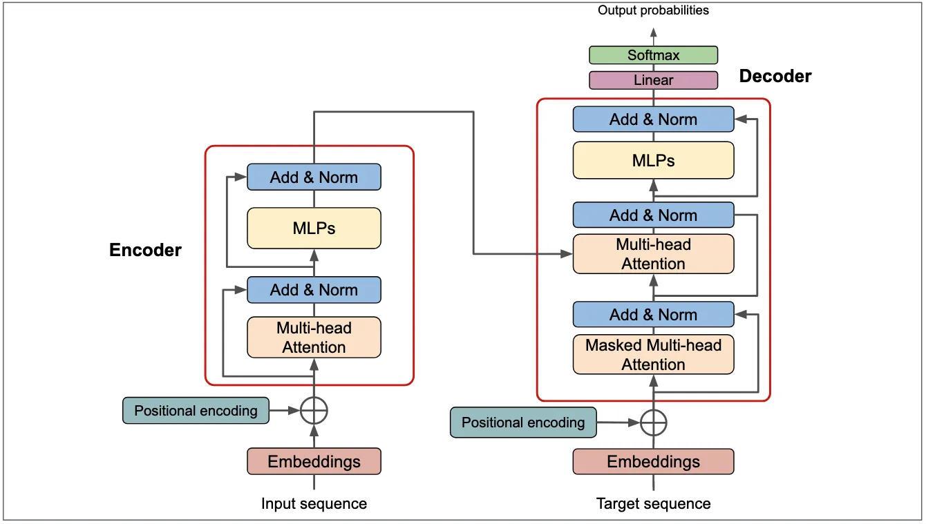
To address these limitations, the Transformer model was proposed. Transformer is composed of multi-head attention, positional encoding, layer normalization, and position-wise feed-forward networks.

Like seq2seq models, Transformer has an encoder and a decoder. The encoder is on the left and the decoder on the right. The core components are multi-head attention and feed-forward networks. A critical element is positional encoding. Since the Transformer does not process tokens sequentially like an RNN, positional information is not implicit in the architecture. The order of tokens is important for meaning, so positional encoding is added to preserve token position information.

Encoder

Multi-Head Attention

Multi-head attention is a central component of Transformer. It extends self-attention. Compared with single-head self-attention, multi-head attention provides two improvements:

• It expands the model's ability to attend to different positions in the input sequence. In single-head self-attention, the final output may be dominated by the query token itself and contain limited information from other tokens.
• It provides multiple subspace representations for attention. With multi-head attention, there are multiple sets of Q, K, and V projection matrices. The original Transformer uses eight heads, so there are eight sets of parameter matrices.

Overall Transformer Structure

The Transformer used for machine translation consists of an encoder and a decoder, each built by stacking identical blocks. Typically, both encoder and decoder contain six blocks. The high-level workflow is:

1. Compute an input representation X for each token by summing token embeddings and positional embeddings.
2. Pass the token representation matrix X (each row is a token representation x) through the encoder. After six encoder blocks, obtain the encoded representation matrix C. X is an n×d matrix, where n is the number of tokens and d is the embedding dimension (the paper uses d = 512). Each encoder block preserves the input dimension.
3. Pass the encoder output matrix C to the decoder. The decoder predicts the next token i+1 conditioned on previously generated tokens 1..i. During generation, future tokens are masked so that predictions do not depend on future positions.

Transformer Input

A token input x in Transformer is the sum of a token embedding and a positional embedding.

Token Embedding

Token embeddings can be obtained via pretraining methods such as Word2Vec or GloVe, or they can be learned within the Transformer during training.

Positional Embedding

Because Transformer does not use an RNN structure, positional information is not inherent and must be provided explicitly. Positional embeddings represent the position of a token in the sequence. Positional embeddings PE have the same dimension as token embeddings and can be either learned or computed by a formula. The Transformer paper uses a fixed, sinusoidal positional encoding given by:

PE(pos, 2i) = sin(pos / 10000^(2i/d))

PE(pos, 2i+1) = cos(pos / 10000^(2i/d))

where pos is the token position, d is the embedding dimension, 2i indexes even dimensions and 2i+1 indexes odd dimensions. This formulation has advantages:

• It generalizes to sequences longer than those seen during training. For a fixed offset k, PE(pos+k) can be computed from PE(pos) using trigonometric identities, enabling the model to represent relative positions.

Self-Attention

Within each encoder block there is a multi-head attention module built from multiple self-attention heads. Decoder blocks contain two multi-head attention modules, one of which is masked. Above each multi-head attention module is an Add & Norm layer: Add refers to the residual connection and Norm refers to layer normalization.

Self-Attention Mechanics

Self-attention computes interactions among tokens using matrices Q (queries), K (keys), and V (values). The input to self-attention is the token representation matrix X or the output of a previous encoder block. Q, K, and V are obtained by applying learned linear projections to the input X.

Computing Q, K, V

Given input matrix X, compute Q = XWQ, K = XWK, V = XWV, where WQ, WK, WV are learned projection matrices. Each row of X, Q, K, V corresponds to one token.

Self-Attention Output

After obtaining Q, K, V, compute the attention scores as QK^T. To avoid large dot-product values, scale by dividing by sqrt(dk) where dk is the key dimension. The resulting n×n matrix represents attention strengths between tokens. Apply softmax row-wise to obtain attention weights, then multiply by V to obtain the final output Z.

Specifically, the output for token 1 is a weighted sum of all token value vectors Vi weighted by the attention coefficients from the first row of the softmax matrix.

Multi-Head Attention

Multi-head attention runs h parallel self-attention layers (heads). Each head receives the same input X but uses different projection matrices, producing outputs Z1...Zh. These outputs are concatenated and passed through a final linear layer to produce the multi-head attention output Z. The output dimension matches the input dimension.

Encoder Block Details

An encoder block consists of: multi-head attention, Add & Norm, position-wise feed-forward network, and another Add & Norm.

Add & Norm

The Add & Norm layer performs a residual connection followed by layer normalization. Given input X, and a sublayer function Sublayer(X) (which can be multi-head attention or feed-forward), the output is LayerNorm(X + Sublayer(X)). Residual connections help with optimization in deep networks by allowing layers to focus on residual changes. Layer normalization standardizes activations within each layer to speed convergence.

Feed-Forward Network

The position-wise feed-forward network consists of two linear layers with a ReLU activation in between. It is applied independently to each position and preserves the input dimension. Formally: FFN(X) = max(0, XW1 + b1)W2 + b2.

Stacking Encoder Blocks

An encoder is formed by stacking multiple encoder blocks. The first encoder block receives the token representation matrix X, each subsequent block receives the previous block's output, and the final encoder output is the encoded representation matrix C used by the decoder.

Decoder

The decoder block resembles the encoder block but includes two multi-head attention modules and a final linear + softmax layer to compute the probability distribution over output tokens. The first multi-head attention in the decoder is masked to prevent positions from attending to subsequent positions during training or autoregressive generation. The second multi-head attention uses the encoder output as K and V, while Q is derived from the previous decoder block output. The final softmax layer computes the probability of the next token.

Masked Multi-Head Attention

Masking ensures that when predicting token i, the model does not have access to tokens i+1 and beyond. For example, when translating "我有一只猫" into "I have a cat", the decoder first inputs a start token and predicts "I", then inputs the start token plus "I" and predicts "have", and so on. Masking enforces the autoregressive property during training.

Summary

• Transformer enables parallelized training compared with RNNs.
• Because Transformer does not inherently encode token order, positional embeddings must be added to the input representations.
• The core of Transformer is the self-attention mechanism; Q, K, V matrices are linear projections of the input.
• Multi-head attention contains multiple self-attention heads, each capturing attention patterns across different subspaces.