Practical Tricks for Reward Models

Overview

A common challenge in RLHF is that the reward model (RM) may be insufficiently accurate to produce the desired results. The two fundamental causes are: 1) low-quality data, and 2) poor model generalization. A technical report from Fudan MOSS addresses both issues and proposes a series of techniques to improve RM performance.

Core Issues

Expanding the two points above:

1. Low-quality data

Errors and ambiguous preference labels in the dataset can prevent the reward model from accurately capturing human preferences. If the training data send mixed signals to the model, the model cannot learn a consistent preference direction.

2. Poor generalization

A reward model trained on a particular distribution may fail to generalize to examples outside that distribution, making it unsuitable for iterative RLHF training. The model may behave very confidently on familiar inputs but fail on unseen cases.

To address these issues, the authors propose methods from two perspectives: data and algorithm.

Data Perspective

In the paper section "Measuring the Strength of Preferences", the authors propose a multi-RM voting method to quantify the strength of preferences in the data. The procedure is:

1. Train multiple reward models: using the same preference dataset but randomizing training order and using different initializations to increase diversity.
2. Compute preference strength: for each pair (for example, two outputs generated by an SFT model), use the reward models to compute each model's score for the two outputs. Then compute the preference strength for each comparison, where r_pos is the score of the selected output and r_neg is the score of the rejected output.
3. Compute mean and standard deviation: use scores from all reward models to compute the mean and standard deviation of preference strength. These statistics help evaluate consistency and strength of preferences.
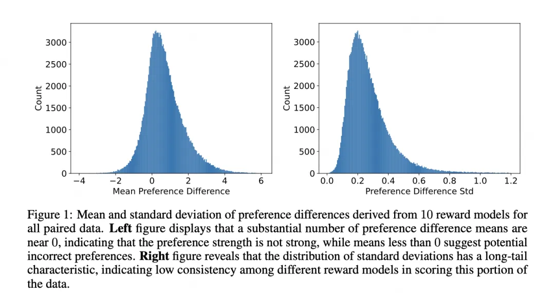
4. Analyze the distribution of preference strength: by examining the distribution of the mean and standard deviation, one can identify erroneous or ambiguous preferences in the dataset. A mean near 0 may indicate incorrect labels; a large standard deviation may indicate unclear preference differences.

The authors provide an example distribution obtained from 10 models for the mean and variance of this metric.

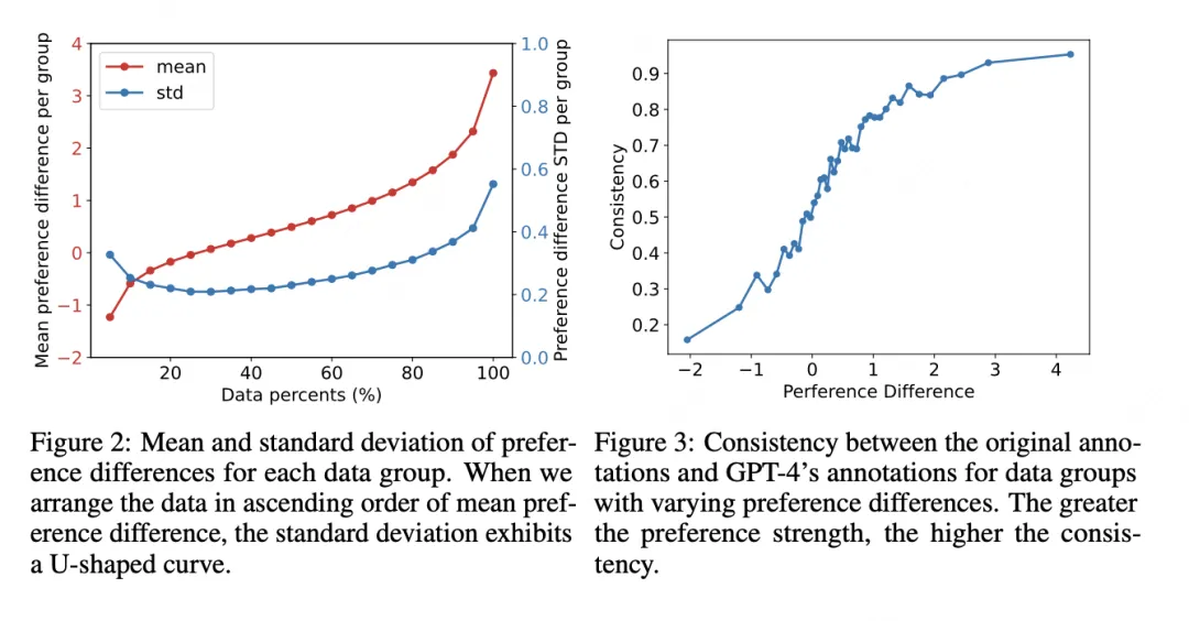
The separation in the data is relatively strong, and as the metric increases, consistency with GPT-4 annotations also increases.

Using this method, the data can be partitioned for analysis into three categories.

1. Negative impact of low-strength preference data: the lowest 20% by preference strength harms validation performance. These examples have mean preference strength below 0, indicating possible incorrect labels.
2. Neutral impact of medium-strength preference data: examples with strength between the 20th and 40th percentiles yield validation accuracy around 0.5 after training. Their mean is near 0, indicating weak preference differences and limited learning signal.
3. Positive impact of high-strength preference data: the remaining 60% significantly improve model performance. However, training only on the top 10% does not yield optimal performance, possibly because those examples are too extreme and cause overfitting.

With quantified preference strength, the dataset can be categorized and different processing strategies applied per category.

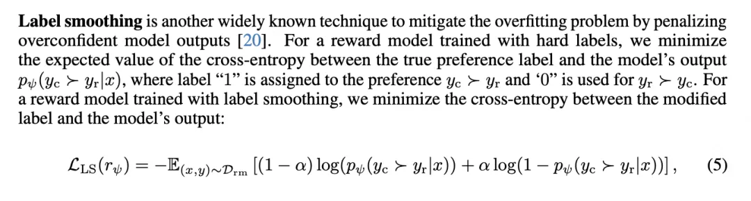
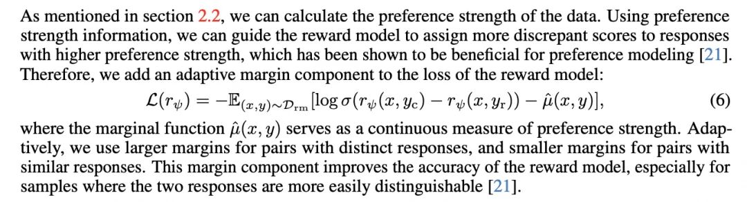
For low-strength data, which likely contains label errors, flipping preference labels can effectively improve model performance. For ambiguous medium-strength data, soft labels and adaptive margins can prevent overfitting. For high-strength data, a combination of soft labels and adaptive margins is particularly effective.

The three specific techniques are: label flipping (invert labels for suspected errors), soft labels (use value-based regression targets instead of hard 0/1 labels, using the measured preference difference as the soft target), and an adaptive margin parameter that scales with the measured preference difference.

An approach to increase intra-class compactness and inter-class separability, inspired by classic methods from face recognition.

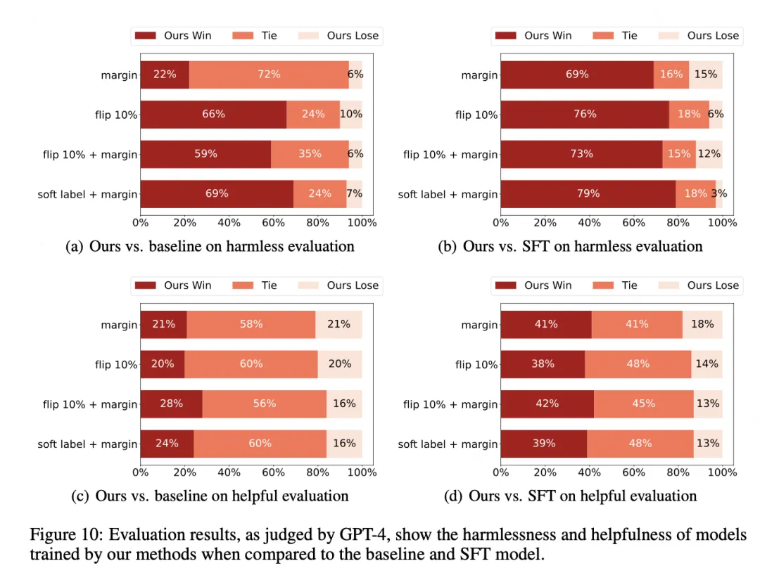
The authors detail experiments measuring reward, loss, perplexity, output length, and other metrics.

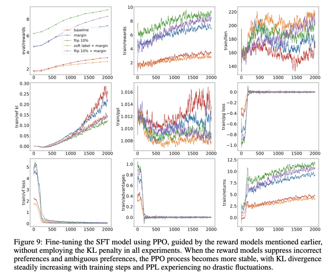
Overall, soft labels are effective for medium-to-high strength preference data, while margin methods work across all strength levels.

Algorithm Perspective

In the paper section "Preference Generalization and Iterated RLHF", the authors propose two main approaches to improve reward model generalization so it can distinguish responses under distribution shifts.

1. Contrastive learning

Integrate a contrastive loss into the reward model training.

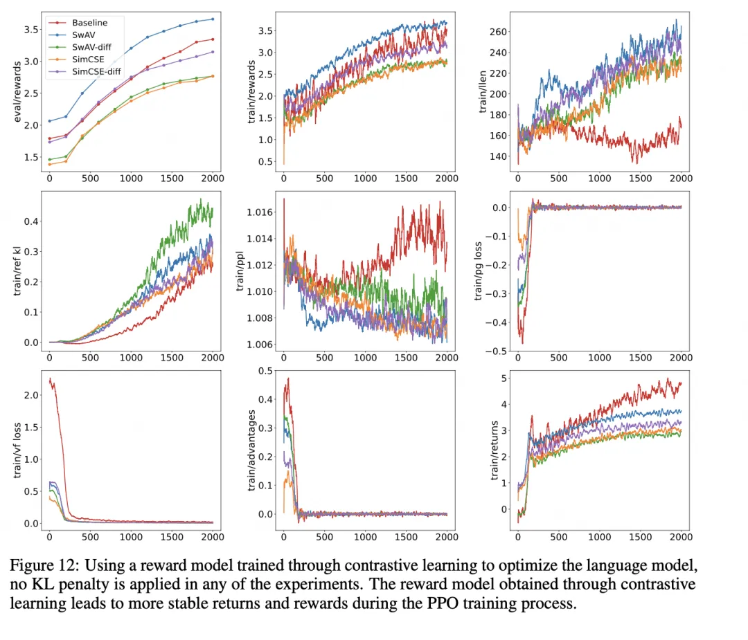
The core question is how to construct the contrastive objective. Two approaches are considered: 1) directly learn representations of preference pairs using standard contrastive learning, and 2) learn the preference difference metric, which is itself a form of contrastive measurement.

The authors evaluate two contrastive methods, swAV and simcse, and cross them with the two learning schemes, producing the experimental results below.

2. Meta Reward Model

The authors propose MetaRM, a meta-learning approach that aligns original preference pairs with distribution shifts. The key idea is to minimize loss on original preference pairs while maximizing discriminative ability on responses sampled from a new distribution.

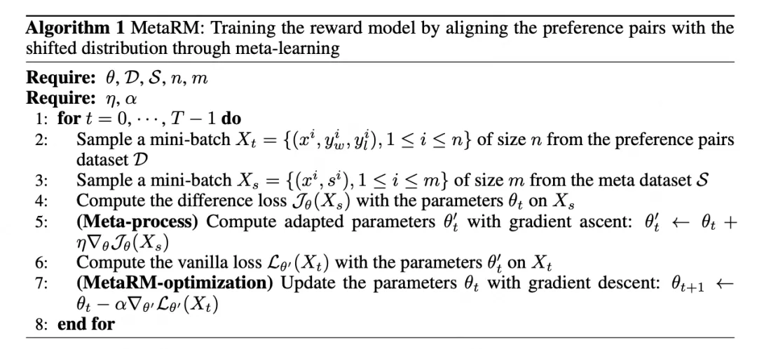
Training process: MetaRM training includes four steps: compute the difference loss on responses sampled from the new distribution, compute gradients of that loss with respect to RM parameters and update parameters, compute original preference pair loss, and compute gradients of that loss with respect to the updated parameters to optimize the original parameters.

The MetaRM algorithm proceeds as follows:

1. Sample a batch from the preference-pair dataset D.
2. Sample a batch from the meta dataset M.
3. Compute the difference loss L_diff on M.
4. Perform a meta-update of the reward model parameters using L_diff.
5. Compute the original loss L_orig on D.
6. Use gradients of L_orig to update the reward model parameters theta_t.

The optimization objective is to maximize the difference loss and minimize the original loss, training the reward model to both fit original preference pairs and adapt to changes in the policy output distribution.

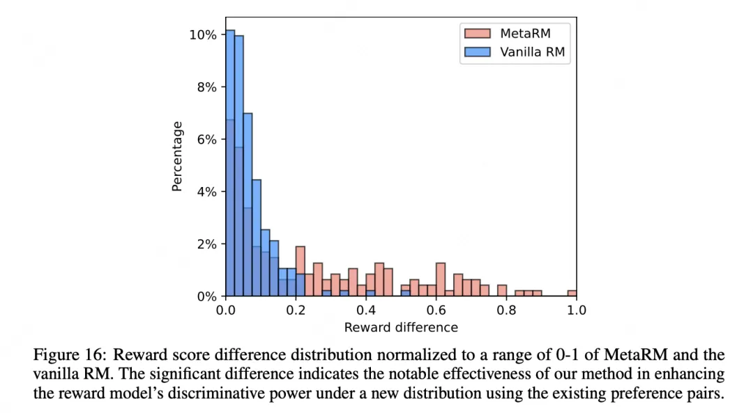
These methods help the reward model capture subtle preference differences and maintain discriminative ability under new distributions, enabling more stable iterative RLHF optimization even when the policy output distribution shifts.

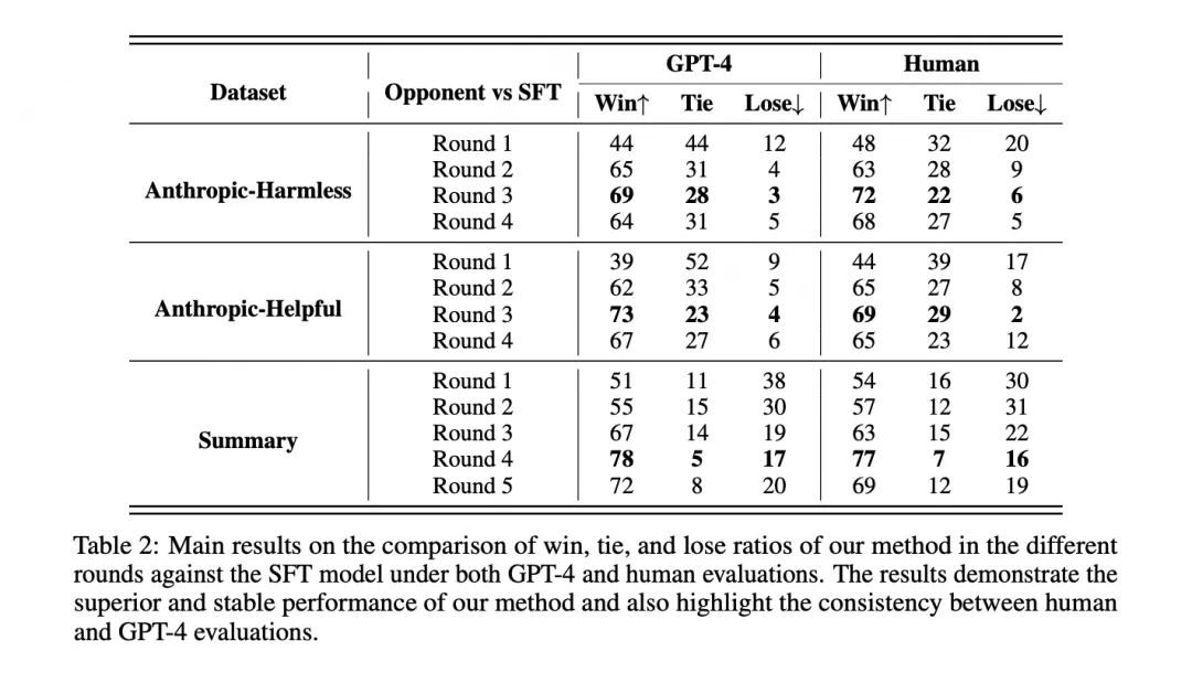
Key experimental results show that MetaRM outperforms baselines on both in-distribution and out-of-distribution evaluations. In in-distribution tasks, MetaRM achieves significantly better performance after several rounds of PPO training.

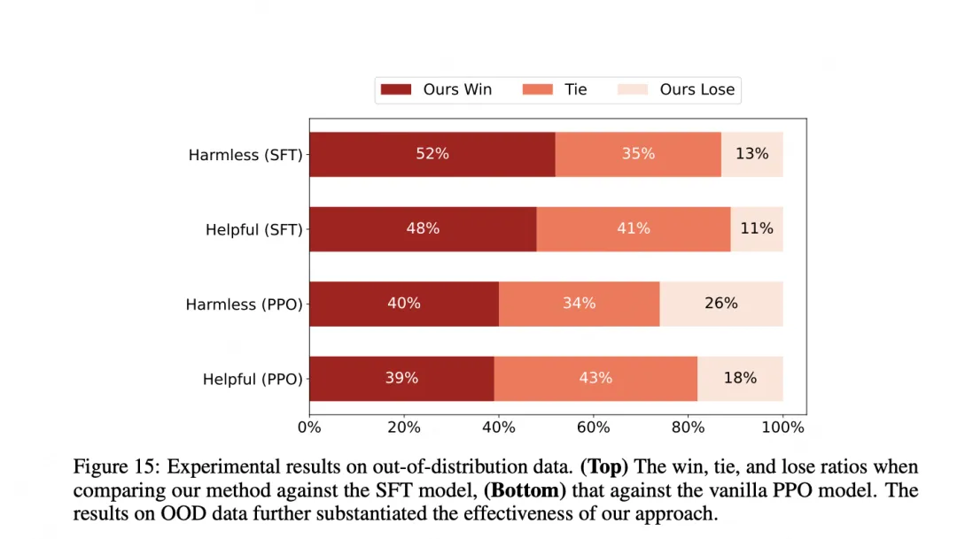
Out-of-distribution analysis shows MetaRM also outperforms baselines on OOD tasks, indicating it can align to new domains without costly relabeling of query sets.

Conclusion

The report proposes a set of methods to address the initial problems of noisy preference data and poor RM generalization. From both data and algorithm perspectives, the authors present practical techniques to improve reward model robustness when handling mislabeled preferences and when adapting to new output distributions.