Optimizing Deep Learning Models

Introduction

This article summarizes common deep learning tuning techniques, including selecting learning rates, weight initialization, and data- and model-level optimizations.

Finding a Suitable Learning Rate

The learning rate is a critically important hyperparameter. Its optimal value depends on model size, batch size, optimizer, and dataset, so it is usually necessary to search for an appropriate learning rate during training rather than rely on intuition.

For example, use fastai's lr_find() to search for a suitable learning rate. The learning rate vs. loss curve below indicates a suitable lr around 1e-2.

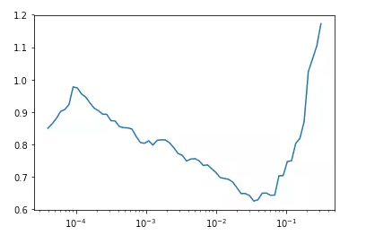
See fastai lead designer Sylvain Gugger's blog "How Do You Find A Good Learning Rate" [1] and the paper "Cyclical Learning Rates for Training Neural Networks" [2].

Learning Rate and Batch Size

Generally, larger batch sizes allow larger learning rates. Intuitively, larger batches provide more reliable gradient estimates, so the optimization direction is steadier; small batches have higher variance and therefore typically require smaller learning rates to avoid instability.

Loss vs. learning rate relationship:

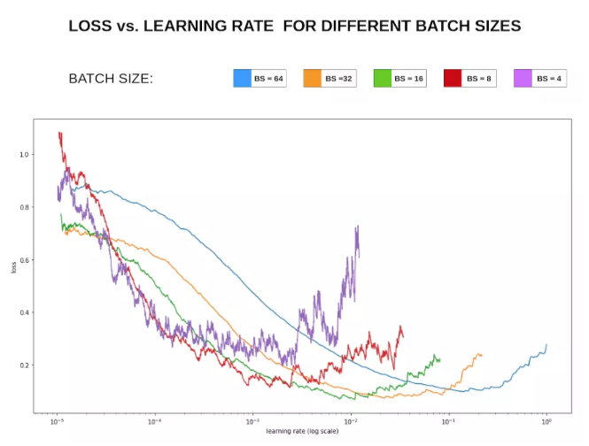
When GPU memory permits, using a larger batch size and then finding a suitable learning rate can speed convergence. Larger batch sizes can also mitigate some batch normalization issues.

Weight Initialization

Weight initialization is less frequently adjusted in practice because many models use pre-trained weights. Initialization is relevant when training from scratch or reinitializing final fully connected layers.

Common initialization methods are kaiming_normal and xavier_normal. Not initializing appropriately can slow convergence or worsen results.

Other methods include Gaussian (normal) initialization and SVD initialization, which can be helpful for RNNs (see https://arxiv.org/abs/1312.6120) [8].

Dropout

Dropout temporarily drops units during training with a given probability. Because dropout is random, each mini-batch effectively trains a different subnetwork. Dropout acts like a bagging ensemble to reduce variance.

Dropout is typically applied to fully connected layers and less often to convolutional layers, since conv layers have fewer parameters. Dropout is not universally beneficial, so apply it judiciously.

Common practice: use higher dropout rates in fully connected layers and lower or no dropout in convolutional layers.

Dataset Handling

Key aspects are data cleaning and data augmentation. fastai's image augmentation pipelines are a common reference for effective augmentation [9].

Hard negative mining: analyze samples the model struggles with and apply targeted methods.

Model Ensembles

Ensembling is a common technique to improve performance and robustness. Typical approaches include:

• Same model and hyperparameters but different initializations.
• Different hyperparameter sets selected via cross-validation.
• Snapshots from different training stages (different iteration checkpoints).
• Different model architectures combined linearly, for example combining RNNs and traditional models.

Common fusion methods:

1. Average model probability outputs from multiple models, then choose final label.
2. Majority voting on labels from multiple models.
3. Aggregate multiple stochastic predictions from each model to produce per-model labels, then vote across models. This leverages variability from unfixed random seeds.

The effectiveness of fusion vs. voting depends on label cardinality and dataset size; experiment to find the best approach.

Differential Learning Rates and Transfer Learning

Transfer learning uses pre-trained models for a target task. When fine-tuning, choosing appropriate learning rates for different layers is important.

Earlier layers typically learn more general features and should use lower learning rates. Later layers, such as final fully connected layers, can use higher learning rates. This technique is called differential learning rates.

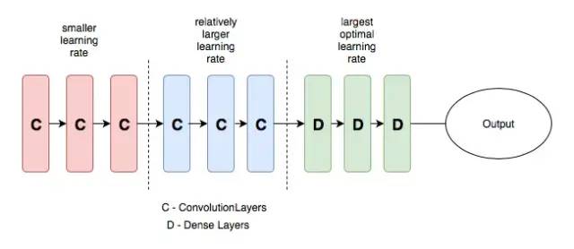
Example learning rate schedule illustration:

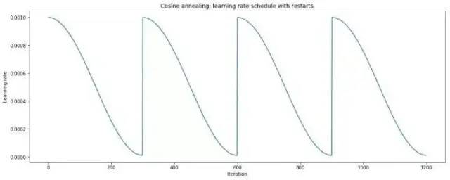
Cosine Annealing and Warm Restarts

Cosine annealing gradually decreases the learning rate following a cosine curve. Warm restarts periodically reset the learning rate to a higher value during training and then continue the annealing. Combining both yields a schedule of decays and restarts.

See SGDR: Stochastic Gradient Descent with Warm Restarts [12] for details.

Overfit a Small Subset

A useful debugging trick is to disable regularization and data augmentation, train on a very small subset of the training data for a few epochs, and verify the model can reach near-zero loss. Failure to do so often indicates implementation issues.

Multi-Scale Training

Multi-scale training feeds images at different resolutions during training. Because convolution and pooling capture multi-resolution features, this can improve performance and help mitigate overfitting when data is limited. Yolo-v2 discussed a similar idea.

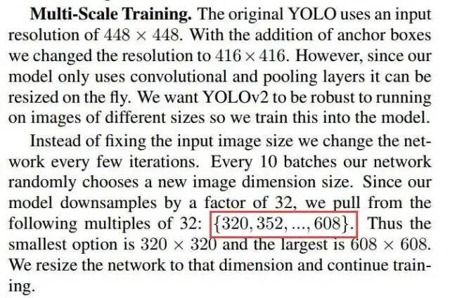
However, multi-scale training is not universally suitable. Inspect transformed images visually to ensure multi-scaling does not destroy important image information.

Cross Validation

Cross validation is often used when data is limited to maximize data reuse. Basic train/validation split is a simple form of cross validation (one-fold). K-fold cross validation, commonly 5-fold, splits data into K parts and rotates the validation fold. Leave-one-out is only practical for very small datasets due to computational cost.

Cross validation applies only to training/validation; the test set should remain separate and is used only for final evaluation.

Optimizers

Choice of optimizer depends on the task. Common choices are Adam and SGD with momentum.

Adam often resolves tricky training issues quickly, but can introduce other behaviors. Some report that SGD yields better generalization after careful tuning. A practical strategy is to run adaptive optimizers initially, then switch to SGD for final convergence. Variants like AdamW or other modifications can address specific issues.

Empirical notes:

• For SGD, start with lr such as 1.0 or 0.1 and halve the learning rate if validation loss stalls.
• On small datasets, SGD sometimes outperforms Adam despite slower initial convergence.
• Adam requires less LR tuning than SGD, but SGD may yield better final solutions if tuned carefully.

Data Preprocessing

Common preprocessing includes zero-centering inputs. PCA whitening is less commonly used.

Training Tips

• Normalize gradients by minibatch size.
• Gradient clipping: cap gradient norm to thresholds such as 5, 10, or 15 to stabilize training.
• Dropout (commonly 0.5) can reduce overfitting on small datasets; using dropout with SGD often shows clear improvements.
• For RNNs, apply dropout at input->RNN and RNN->output connections. See relevant literature on dropout for RNNs [15].
• Avoid sigmoid activations except where needed to constrain outputs; prefer tanh or ReLU to reduce vanishing gradients. Sigmoid has significant gradient only in a limited range.
• Embedding sizes and RNN hidden dimensions often start around 128 and are tuned from there. Batch size tuning is important; larger is not always better.
• Initializing word embeddings with pretrained word2vec can improve convergence and final results on small datasets.
• Shuffle training data whenever possible.
• Initialize LSTM forget-gate bias to 1.0 or larger to improve convergence in many tasks [16].
• Batch normalization often improves training stability and performance.
• If an MLP has equal input and output sizes, consider a Highway Network as a potential refinement [17].
• Alternating regularization every other epoch is a heuristic some practitioners use.
• When dataset is very large, run quick experiments on 1/100 or 1/10 of the data to estimate model behavior and training time before full-scale runs.
• If GPU runs produce unhelpful error messages, try rerunning on CPU to get clearer diagnostics. For example, "Model diverged with loss = NaN" can indicate out-of-range input IDs for a softmax vocabulary.
• To find a good initial learning rate, start from a very small value (e.g., 1e-7) and exponentially increase it each step (e.g., multiply by 1.05). After a few hundred steps, identify the learning rate range where loss decreases most rapidly.
• As an RNN regularizer, batch size = 1 can act as a strong regularizer in some tasks, although it increases runtime.
• Maintain reproducibility and good experiment logging to enable reliable analysis of results.

Final Notes

Among hyperparameters, learning rate is the most important—familiarize yourself with cosine learning rate schedules and cyclic learning rates. Next priorities include batch size and weight decay. Once the model performs reasonably, data augmentation and loss function adjustments can provide further improvements.