ALLPCB


1. Parameter provenance and test conditions
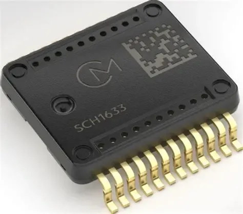
The SCH1633 nominal G-sensitivity value of 0.0005 (deg/s)/g must be interpreted within its test reference frame and conditions. If the datasheet does not state them explicitly, the following assumptions are typically implied:
Acceleration condition: The value is usually measured under a constant 1 g acceleration. Therefore the G-sensitivity coefficient is 0.0005 deg/s per g.
Directionality: The term "typical value" strongly suggests the measurement was taken on the axis of least G sensitivity (often selected during factory screening), or in a test orientation that removes Earth rotation effects (for example, rotation-table polar axis). This implies:
- Significant anisotropy: The sensor's G sensitivity on other axes may be much higher than the typical figure, possibly approaching the stated maximum values.
- Application risk: If the actual installation orientation differs from the test orientation, performance may degrade unexpectedly.
Frequency dependence: G sensitivity often varies with vibration frequency. The typical value is likely measured in quasi-static conditions or at a single low frequency. Sensor response under wideband vibration (for example, engine harmonics) can differ substantially and should be evaluated with the vibration rectification error (VR) parameter.
2. Quantitative error modeling
Substituting the parameter into inertial navigation error dynamics quantifies the impact.
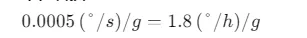
Unit conversion:
0.0005 deg/s per g = 1.8 deg/h per g.
Error propagation:
Under a sustained acceleration a (in g), the angular rate error is:
delta_omega = 0.0005 * a deg/s = 1.8 * a deg/h.
Integrating this error over time t (hours) produces an attitude angle error approximately:
delta_angle ≈ 1.8 * a * t deg.
Typical scenarios and examples:
- Drone maneuvering: During a 5 g aggressive maneuver, the instantaneous false angular rate equals 0.0005 * 5 = 0.0025 deg/s, which equals 9.0 deg/h. If this persists for 10 seconds (≈0.00278 h), it yields about 0.025 deg instantaneous attitude error.
- Long-range flight navigation: A persistent 0.02 g acceleration during a 10-hour flight accumulates approximately 1.8 * 0.02 * 10 = 0.36 deg of attitude error. This approaches the tolerance limit for pure-inertial segments of precision approaches.
- Vibration environments: Wideband vibration with 1 g RMS can cause rectification effects that generate steady-state bias comparable to the typical value, disrupting control systems.
3. Positioning within sensor technology tiers
Comparing major gyro technology tiers clarifies SCH1633's market and technical positioning.
| Performance level | Typical technology | G-sensitivity range | SCH1633 position | Applications |
|---|---|---|---|---|
| Navigation grade | Fiber optic gyro (FOG), ring laser gyro (RLG) | < 0.001 deg/h per g | Far superior to SCH1633 | Submarines, strategic missiles, spacecraft |
| Tactical grade | High-precision MEMS, mid-range FOG | 0.01 - 0.1 deg/h per g | Near the upper bound | Tactical missiles, drones, attitude reference systems |
| Industrial grade | Commercial MEMS | 0.1 - 10 deg/h per g | Core range (1.8 deg/h per g) | Robotics, stabilized gimbals, AGV |
| Consumer grade | Smartphone MEMS | > 10 deg/h per g | Far better than consumer level | Phones, game controllers, wearables |
Conclusion: The SCH1633 sits at the high end of industrial performance and the low end of tactical performance. It outperforms typical industrial sensors but is not sufficient for standalone tactical-grade navigation.
4. System-level compensation strategies and limits
To build a reliable system with SCH1633, the following architecture strategies are required to mitigate G-sensitivity limitations.
Multi-sensor tightly coupled architecture:
- Accelerometer-aided compensation: Read three-axis accelerometer data in real time and model delta_omega = f(ax, ay, az), typically using first- or second-order polynomial models, then subtract G-related bias in software dynamically.
- GNSS assistance: Use satellite-derived velocity and position to periodically reset accumulated inertial solution errors and limit divergence. Applicable for drones and vehicle navigation.
- Magnetometer assistance: Provide absolute heading reference to correct slow yaw drift.
Hardware design and calibration enhancements:
- Six-face calibration method: Test all six faces under +1 g and -1 g to fit a full 3x3 G-sensitivity coefficient matrix rather than relying on a single typical value.
- Vibration isolation: Use damping materials in mechanical mounting to filter high-frequency vibration input and reduce vibration rectification error.
- Temperature compensation: G-sensitivity coefficients vary with temperature and require temperature-dependent calibration.
5. Selection recommendations
Consider SCH1633 only when:
- System dynamics are high but pure-inertial navigation intervals are short (< 1 minute), or there are frequent external observations (optical or satellite) for correction.
- Cost constraints are significant and attitude accuracy requirements are on the order of 0.1 to 1.0 deg rather than 0.01 deg.
- Primary use cases are attitude stabilization and control (for example, gimbals and robot balancing) rather than autonomous precision navigation and positioning.
- Engineering resources are available for comprehensive field calibration and compensation, and the team can accept directional performance variation.
Summary: The SCH1633 is a sensor with clearly defined performance under specific conditions. Its 0.0005 deg/s per g G-sensitivity indicates potential as a high-performance industrial device in controlled dynamic environments, while also defining the technical boundary before it can be used in long-endurance, high-precision navigation. Successful applications depend on understanding the underlying physics and implementing system-level compensation to achieve an optimal balance between cost and performance.