ALLPCB


Overview
This article provides a detailed explanation of Legendre filter synthesis, showing how the Legendre filter is derived from the monotone minimum-attenuation constraints. It also describes a MATLAB-based filter design tool and demonstrates its use with low-pass and band-pass examples. The MATLAB source code is available on GitHub.

Legendre Filter Characteristics and Uses
The Legendre filter (also known as the Papoulis filter or L filter) was proposed by Papoulis in 1959. Its magnitude response lies between the Butterworth and Chebyshev type I responses: monotonic in the passband like a Butterworth filter (no passband ripple), while achieving a steeper stopband roll-off similar to a Chebyshev filter. Despite these properties, Legendre filters are relatively uncommon in practical applications.
Legendre Approximation and Design Constraints
The design uses a characteristic polynomial and the overall filter magnitude expression. The constraints considered are:
- The characteristic is an nth-order polynomial (realizability; zero gain at infinite frequency).
- Low-pass definition: the gain at frequency 0 equals the specified passband reference.
- Definition of the low-pass bandwidth.
- No ripple in the passband over the interval [0,1] (Legendre filter property).
- Maximum attenuation rate at the cutoff frequency (Legendre filter property).
No ripple means the amplitude function is monotonic on [0,1]. The maximum attenuation condition can be expressed as the derivative having its maximum magnitude at the cutoff point.
Study of the Derivative of the Characteristic Polynomial
Because constraints 4 and 5 relate to monotonicity and steepest decay, it is convenient to study the derivative of the characteristic polynomial. This reformulation leads to finding a polynomial whose square integrates to a given value over the design interval. For odd-order Legendre filters the characteristic polynomial can be expressed as a perfect square of another polynomial, so the problem reduces to finding a function whose square integrates to a known value on [0,1].
Direct Optimization Example
If Legendre or Jacobi polynomials are not used, a direct polynomial optimization can be performed numerically. As an example for a 5th-order case, assume the derivative of the sought polynomial is of the form of a polynomial that is nonnegative on [0,1], which satisfies the monotonic condition. Then the integral constraint must be met. The resulting optimization is multi-parameter and can be solved by standard numerical methods. For example, using a numerical optimizer:
NMaximize[{(a0 + a1 + a2)^2, Integrate[2*x*(a2*x^4+a1*x^2 + a0)^2, {x, 0, 1}] == 1}, {a0, a1, a2}];
Solving this yields the final 5th-order Legendre characteristic polynomial.
Orthogonal Polynomial Approach
Orthogonal polynomials are convenient because individual orthogonal terms do not interfere with each other, allowing independent adjustment of coefficients for approximation purposes.
Legendre Polynomial Approximation
Papoulis used Legendre polynomials to form the approximation. Legendre polynomials are a family of orthogonal polynomials. The characteristic polynomial can be expressed as a combination of Legendre polynomials, which simplifies the integral expressions because cross terms integrate to zero over the symmetric interval.
Shifted Jacobi Polynomial Approximation
Fukada used shifted Jacobi polynomials for approximation. Shifted Jacobi polynomials are also orthogonal and include two parameters; varying those parameters yields different characteristic shapes. The shifted Jacobi polynomials include Legendre polynomials as a special case when the parameters are equal. The orthogonality property and weighting function provide flexibility to design different filter characteristics by choosing appropriate parameter values.
Interpretation of the Weight Function
For Legendre polynomials the weight function is constant on the interval [-1,1], meaning all points contribute equally to the integral. Under the squared-function constraint, any passband ripple increases the integral compared with a flat response, so the constrained optimum under a constant weight yields a monotonic, no-ripple passband.
Evaluation of Legendre Filters
After Papoulis introduced this class of monotone-response filters, several related monotone filter designs appeared, including LSM (Least-Squares-Monotonic) and H filters. They differ mainly in the specific form of constraint 5. For example:
- H filter: modify constraint 5 so the response decays fastest at the asymptotic frequency point (equivalently maximizing the highest coefficient of the characteristic polynomial).
- LSM filter: modify constraint 5 so the area enclosed by the passband curve is minimized (equivalently minimizing passband reflection or insertion loss across the passband).
- Butterworth filter: modify constraint 5 so the response is flattest at frequency 0.
These design alternatives show that Papoulis' formulation provides a unifying framework for several monotone-response filters. Some recent papers argue that beyond the specific roll-off behavior, Legendre filters offer no clear advantage over classical designs in practical terms; interested readers can consult comparative studies of Papoulis and Chebyshev filters.
Coefficients, Poles, and Zeros
There is no single closed-form formula for Legendre characteristic polynomials for all orders, but coefficients can be computed numerically. The MATLAB implementation below generates these coefficients; the returned vector is ordered from lowest to highest degree.
%--------------------------------------------------------------------------
% Edited by bbl
% Date: 2023-06-11(yyyy-mm-dd)
% Legendre filter coefficient design
% Note: return value ordered from low degree to high degree
%--------------------------------------------------------------------------
function [Ln] = funGenLegendreCharacteristicPoly(FilterOrder)
% Initialize coefficient vector
coefficients = ((1:FilterOrder).*2 - 1);
% Define coefficient for normalization
if mod(FilterOrder, 2) == 1
    % Odd polynomial order
    half_order = (FilterOrder - 1) / 2;
    norm_coefficient = 1 / (sqrt(2 * (half_order + 1) * (half_order + 1)));
else
    % Even polynomial order
    half_order = FilterOrder / 2 - 1;
    norm_coefficient = 1 / sqrt((half_order + 1) * (half_order + 2));
    % Check if the half_order is odd or even
    if mod(half_order, 2) == 1
        % Odd
        coefficients(1:2:end) = 0;
    else
        % Even
        coefficients(2:2:end) = 0;
    end
end
% Apply normalization to coefficients
coefficients = coefficients * norm_coefficient;
% Initial value for the Phi
Phi = 0;
% Generate polynomial and add to Phi
for i = 1:half_order + 1
    current_coefficient = coefficients(i);
    legendrePoly = JacobiPoly(i - 1, 0, 0); % Gen legendre polynomial
    Phi  = polyadd(Phi, current_coefficient * legendrePoly);
end
% Calculate Phi^2
Phi_squared = conv(Phi, Phi);
% For even polynomial order, multiply Phi_squared by (x+1)
if mod(FilterOrder, 2) == 0
    Phi_squared = conv(Phi_squared, [1,1]);
end
% Calculate the integral of Phi_squared
integral_of_Phi_squared = polyint(Phi_squared, 0);
% Define the range for polyval function
lower_range = -1;
upper_range = [2, -1];
% Calculate polyval for lower and upper ranges
D = polyval(integral_of_Phi_squared, lower_range);
U = substitute_poly(integral_of_Phi_squared, upper_range);
% Final result
Ln0 = polyadd(U, -D);
nLn = length(Ln0);
Ln = zeros(1, nLn*2-1);
Ln(3:2:end) = fliplr(Ln0(1:end-1));
Ln(1)     = Ln0(end);
end
> [Ln] = funGenLegendreCharacteristicPoly(5)
Ln =
    0   0   1   0   -8  0   28  0   -40 0   20
The result above is the 5th-order Legendre characteristic polynomial coefficients in polynomial form.
Frequency Response, Poles, and Synthesis
Numerical results for the first several orders indicate that the Legendre frequency response lies between Butterworth and Chebyshev responses. In practice, comparisons often show Legendre filters do not outperform Chebyshev filters in roll-off efficiency, which is why some researchers consider them more of academic interest.
Left-half-plane poles for the first several orders produce the standard all-pole realizations. Zero-pole plots show Legendre poles distributed approximately on an ellipse between the Butterworth and Chebyshev pole distributions. By varying Chebyshev ripple, the Legendre pole distribution can be seen as intermediate between the two.
Synthesis Example
Legendre filter synthesis is similar to Butterworth synthesis because both are all-pole designs. A simple 3rd-order Legendre filter synthesis example can be constructed from the computed poles and standard low-pass network transformations.
MATLAB-Based Filter Design Tool
A MATLAB app was developed to support design and analysis of various filter types. Features include:
- Support for Legendre, Gaussian, Bessel, Elliptic/Cauer, Chebyshev I, Inverse Chebyshev (Chebyshev II), and Butterworth designs.
- Support for four passband types: LPF, HPF, BPF, BRF.
- Switchable T and PI network topologies.
- Ability to specify stopband attenuation to determine filter order.
- Ability to specify passband attenuation for synthesis.
- Configurable source and load terminations, including resistor, current source, open, and short options.
- Amplitude-frequency response, pole-zero analysis, and transient analysis capabilities.
- Display of ideal frequency response, pole-zero map, and simulated frequency response from circuit simulation.
- Support for approximating with real standard components.
Design Examples
Legendre LPF design example: a 7th-order low-pass Legendre filter with a -3 dB cutoff at 1 GHz, 50 ohm input and output terminations. The design process yields the final component values and simulation plots for transient and AC analysis.
Legendre BPF design example: a 6th-order band-pass Legendre filter centered at 1 GHz with 1 GHz bandwidth, 50 ohm input and high-impedance output. The design includes transient and AC simulation results.
Code Availability
The MATLAB source code for the design tool and coefficient generation routines is hosted on GitHub.
Preview: Linear-Response Filter Design
Returning to the initial topic of passive analog filter design, a linear-response filter is another form of monotone-response filter where the magnitude response follows a linear slope on the normalized frequency interval. Design constraints for a linear-response low-pass filter can be stated similarly:
- The characteristic is an nth-order polynomial (realizability).
- The response at frequency 0 equals the specified insertion loss IL.
- The response at normalized frequency 1 equals unity (maximum value).
- No ripple on the interval [0,1] (linear response property).