Core Principles of Major Machine Learning Models

Introduction

In simple terms, a machine learning model is a mathematical function that maps input data to predicted outputs. More specifically, a machine learning model adjusts its parameters by learning from training data to minimize the error between predicted outputs and true labels.

There are many types of models in machine learning, such as logistic regression, decision trees, and support vector machines. Each model has suitable data types and problem domains. Different models also share many commonalities and can be linked through transformations or extensions.

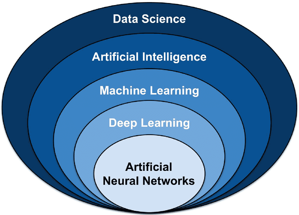
For example, starting from the connectionist perceptron, adding hidden layers transforms it into a deep neural network. Introducing a kernel function to a perceptron-like structure leads to SVM. These transformations illustrate intrinsic relationships among models. For convenience, the models are roughly categorized into the following six classes to highlight basic commonalities and analyze each class in depth.

1. Neural Network (Connectionist) Models

Connectionist models simulate brain neural network structures and functions. Their basic unit is the neuron, which receives inputs from other neurons and adjusts weights to change input influence. Neural networks are often treated as black boxes; with multiple nonlinear hidden layers they can approximate a wide range of functions.

Representative models include DNN, SVM, Transformer, and LSTM. In some cases, the final layer of a deep neural network can be viewed as a logistic regression model used for classification. Support vector machines can be regarded as a special type of neural architecture with essentially two layers—input and output—while the kernel function enables complex nonlinear transformations similar to deep networks.

Deep neural networks (DNN) consist of multiple layers of neurons. Through forward propagation, input data is passed through each layer and transformed to produce outputs. Each layer receives outputs from the previous layer as input and forwards its output to the next layer. DNN training uses the backpropagation algorithm: compute the error between the output layer and true labels, propagate the error backward through the layers, and update weights and biases via gradient descent. Iterating this process optimizes the network parameters to minimize prediction error.

DNN advantages include strong feature learning capability and high model expressiveness without manual feature design. Disadvantages include large parameter counts that can lead to overfitting, high computational cost, long training times, and limited interpretability. Example Python code using Keras to build a simple DNN:

from keras.models import Sequential from keras.layers import Dense from keras.optimizers import Adam from keras.losses import BinaryCrossentropy import numpy as np # Build model model = Sequential() model.add(Dense(64, activation='relu', input_shape=(10,))) # Input layer has 10 features model.add(Dense(64, activation='relu')) # Hidden layer has 64 neurons model.add(Dense(1, activation='sigmoid')) # Output layer has 1 neuron, using sigmoid activation for binary classification # Compile model model.compile(optimizer=Adam(lr=0.001), loss=BinaryCrossentropy(), metrics=['accuracy']) # Generate synthetic dataset x_train = np.random.rand(1000, 10) # 1000 samples, each with 10 features y_train = np.random.randint(2, size=1000) # 1000 labels for binary classification # Train model model.fit(x_train, y_train, epochs=10, batch_size=32) # Train for 10 epochs with batch size 32

2. Symbolic Models

Symbolic models are based on logical reasoning and treat cognition as symbol manipulation. They encode information as identifiable symbols and apply explicit rules to manipulate those symbols using rule bases and inference engines. Representative systems include expert systems, knowledge bases, and knowledge graphs. A simple expert system example:

# Define rule base rules = [ {"name": "rule1", "condition": "sym1 == 'A' and sym2 == 'B'", "action": "result = 'C'"}, {"name": "rule2", "condition": "sym1 == 'B' and sym2 == 'C'", "action": "result = 'D'"}, {"name": "rule3", "condition": "sym1 == 'A' or sym2 == 'B'", "action": "result = 'E'"},] # Define inference engine def infer(rules, sym1, sym2): for rule in rules: if rule["condition"] == True: # Execute action when condition is true return rule["action"] return None # Return None when no rule satisfies conditions # Test expert system print(infer(rules, 'A', 'B')) # Output: C print(infer(rules, 'B', 'C')) # Output: D print(infer(rules, 'A', 'C')) # Output: E print(infer(rules, 'B', 'B')) # Output: E

3. Decision Tree Models

Decision trees are nonparametric methods for classification and regression, representing decisions via a tree structure. Mathematically, tree models can be seen as piecewise functions. They use entropy and related measures from information theory to select optimal split attributes and construct trees with good classification performance.

Decision trees recursively split the dataset into subsets until each subset belongs to a single class or meets stopping criteria. Splits are evaluated using measures such as information gain, gain ratio, or Gini index to choose the best attribute. Classic algorithms include ID3, C4.5, and CART. ID3 uses information gain; C4.5 improves ID3 by using gain ratio and pruning; CART uses the Gini index and can handle continuous and ordinal attributes.

Example using scikit-learn to build a CART decision tree:

from sklearn.datasets import load_iris from sklearn.model_selection import train_test_split from sklearn.tree import DecisionTreeClassifier, plot_tree # Load dataset iris = load_iris() X = iris.data y = iris.target # Split training and test sets X_train, X_test, y_train, y_test = train_test_split(X, y, test_size=0.2, random_state=42) # Build decision tree model clf = DecisionTreeClassifier(criterion='gini') clf.fit(X_train, y_train) # Predict test set y_pred = clf.predict(X_test) # Visualize decision tree plot_tree(clf)

4. Probabilistic Models

Probabilistic models use probability theory to describe distributions of random phenomena and their relationships. They employ probability distributions for random variables and conditional probability rules to model dependencies. Probabilistic models support quantitative analysis and prediction of stochastic events.

Representative models include naive Bayes classifiers, Bayesian networks, and hidden Markov models. Naive Bayes and logistic regression both rely on probabilistic reasoning; hidden Markov models and Bayesian networks model sequences and dependencies among variables.

Example using scikit-learn to implement a Gaussian naive Bayes classifier:

from sklearn.datasets import load_iris from sklearn.model_selection import train_test_split from sklearn.naive_bayes import GaussianNB # Load dataset iris = load_iris() X = iris.data y = iris.target # Split training and test sets X_train, X_test, y_train, y_test = train_test_split(X, y, test_size=0.2, random_state=42) # Build Gaussian Naive Bayes classifier clf = GaussianNB() clf.fit(X_train, y_train) # Predict test set y_pred = clf.predict(X_test)

5. Nearest Neighbor Models

Nearest neighbor models are nonparametric methods for classification and regression based on instance-based learning. They determine similarity between data points by measuring distances in feature space. They do not require explicit model training in the conventional sense.

The K-nearest neighbors (KNN) algorithm classifies a sample based on the majority label among its k nearest training samples in feature space. Variants include weighted KNN, multi-level classification KNN, radius search, K-means, and approximate nearest neighbor (ANN) algorithms.

ANN methods trade some accuracy for improved time and space efficiency when searching nearest neighbors in large datasets by allowing approximate results to reduce search time.

Example using scikit-learn to implement KNN:

from sklearn.datasets import load_iris from sklearn.model_selection import train_test_split from sklearn.neighbors import KNeighborsClassifier # Load dataset iris = load_iris() X = iris.data y = iris.target # Split training and test sets X_train, X_test, y_train, y_test = train_test_split(X, y, test_size=0.2, random_state=42) # Build KNN classifier knn = KNeighborsClassifier(n_neighbors=3) knn.fit(X_train, y_train) # Predict test set y_pred = knn.predict(X_test)

6. Ensemble Learning Models

Ensemble learning is a methodology that combines multiple learners to improve overall prediction accuracy and stability by aggregating their outputs. The core idea is that combining multiple base learners can reduce variance and bias, improving generalization. Introducing diversity among base learners—via different algorithms, data, or parameters—often improves ensemble performance.

Common ensemble methods include bagging, boosting, and stacking. Bagging introduces diversity and reduces variance to improve stability and generalization. Boosting changes the weighting of base learners to improve performance. Stacking arranges base learners into a layered structure and uses a meta-learner to integrate their predictions.

Representative ensemble models include random forest, isolation forest, GBDT, AdaBoost, and XGBoost. Example using scikit-learn to implement a random forest classifier:

from sklearn.ensemble import RandomForestClassifier from sklearn.datasets import load_iris from sklearn.model_selection import train_test_split # Load dataset iris = load_iris() X = iris.data y = iris.target # Split training and test sets X_train, X_test, y_train, y_test = train_test_split(X, y, test_size=0.2, random_state=42) # Build random forest classifier clf = RandomForestClassifier(n_estimators=100, random_state=42) clf.fit(X_train, y_train) # Predict test set y_pred = clf.predict(X_test)

Conclusion

By grouping models with similar principles into categories, we can systematically explore their mechanisms and interconnections to gain a more comprehensive understanding of model behavior and relationships.