ALLPCB


Overview
Near-field probes are a basic tool in EMC diagnosis and design. EMC engineers use near-field probes to relate near-field electromagnetic emissions to far-field radiated fields for comparative analysis, to identify critical subcomponents in complex systems, and to combine spectrum and time-domain waveforms without contacting the circuit. Experienced engineers can also use probes to inject specific RF energy into the near field to analyze immunity issues. Near-field probes are convenient, safe, and efficient, making them a common instrument in an EMC engineer's toolkit.
Market probe specifications and limitations
Although widely used, near-field probes are auxiliary tools rather than standardized test equipment defined by EMC test or certification standards. As a result, probe performance, specifications, and calibration methods lack standardization. Many probe models and types are available on the market, but vendor data sheets often lack sufficient frequency response and coupling information. Such data can support coarse detection but do not enable quantitative near-field electromagnetic measurements.
Most electric-field probe vendors do not provide the frequency response and coupling curves that users most often require.
Calibration results from metrology labs
Many probes are submitted to calibration laboratories to meet equipment management requirements. Without standardized procedures, the submitter or the laboratory must decide the calibration method. Some laboratories have adapted power-probe calibration methods and produced curves like the one below.
That laboratory used a TEM cell, a power probe, and a network analyzer to perform a substitution calibration: a power probe established a reference in the TEM cell and the network analyzer normalized the measurement; the near-field probe was then substituted for the power probe to derive an electric-field calibration curve. This substitution method, designed for isotropic power probes, is not ideal for directional near-field probes. Directional probes, such as loop magnetic probes with sensing area around the ring, rod probes sensing at the tip, or shovel-shaped E-field probes sensing on an inclined surface, may not achieve optimal directional coupling in a TEM cell, affecting calibration results. Additionally, TEM cell calibrations in some labs may stop at 100 MHz and thus do not cover the full frequency range of many near-field probes. GTEM cells can extend calibration frequency, but limitations remain for many submitted calibrations.
A paired-probe calibration method
Because vendor information is limited and metrology lab curves rarely provide the probe coefficients EMC engineers need, a practical calibration approach is useful for guiding probe use. Near-field probes are simple devices comprising a sensing element, a balun (unbalanced-to-balanced converter), insulating packaging, and a coaxial connector, so manufacturing consistency within a model and batch is typically high. If we assume that probes of the same model and batch have identical coupling coefficients, and that transmit and receive attenuation are symmetric, we can measure the combined coefficient of two probes to infer the single-probe coefficient. Paired-probe calibration can be performed using a network analyzer measuring S21 or with a spectrum analyzer equipped with a tracking generator and receiver.
Calibration using a spectrum analyzer with tracking generator
A spectrum analyzer with a tracking generator is a more common EMC instrument than a network analyzer and is well suited to calibrating various probes. The following steps describe a paired-probe calibration method using a spectrum analyzer with tracking generator and present measured results.
Step 1: Setup and cable normalization
Set frequency and bandwidth, enable the tracking generator, short the coaxial cable, calibrate the cable, and normalize the cable response.
Step 2: Measurement settings
Set the Y axis to dBμV, ensure at least 80 dB measurement depth, and place the normalized cable curve at the top of the display.
Step 3: Measure paired probes
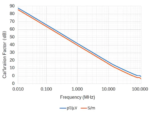
Connect the probe pair and ensure maximal mutual coupling between the probes. The spectrum analyzer will display the second curve; the difference between the normalized reference and this curve is insertion loss. Half of the insertion loss corresponds to the single probe's conversion coefficient for the planar electric field.
The tracking generator signal travels from the RF output port to the spectrum analyzer RF input after two attenuations by the probe pair. In logarithmic units (dB), the attenuation multiplies, so the single-probe attenuation in dB is half the measured S21 insertion loss in dB.
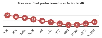
The calculated single-probe curve characterizes the frequency response and coupling on the probe sensing surface. This coefficient can be used to convert detected signals to RF field magnitudes on the sensing plane. A logarithmic frequency axis is more suitable than a linear axis for wideband displays. The example curve shows a 6 dB attenuation across 30–120 MHz, a 6 dB flatness bandwidth roughly from 10 MHz to 300 MHz, making the probe suitable for both radiated and conducted signal detection. Note that a resonance notch appears after about 500 MHz, so measurements above 500 MHz with this probe require caution.
This paired-probe method effectively measures probe frequency response and identifies the probe's application band and sensitivity.
Different probe types have different frequency responses and coupling coefficients. This calibration method allows quantifying probe coefficients across relevant bands so engineers can select appropriate probes for specific applications.
Calibration for RF near-field injection (immunity testing)
Experienced EMC engineers use near-field probes to inject near-field interference into devices under test to identify immunity weaknesses at the PCB and circuit level, such as EFT burst immunity, radiated immunity, and conducted immunity diagnostics. For injection use, probe impedance, power handling, and near-field coupling capability are key parameters.
Probe impedance should match the RF power source output to maximize injection and protect the signal source and power amplifier. Probes should be near 50 ohms; large mismatches require attenuators for matching. Use a vector network analyzer to perform single-port S11 impedance calibration. Power handling is also important: excessive injection power into magnetic probes can cause magnetic saturation or damage. Near-field coupling for injection follows the same insertion loss behavior measured during probe detection calibration: stronger detection coupling implies stronger injection capability.
Conclusion
Paired-probe calibration provides a fast and practical way to obtain frequency response and coupling curves for near-field probes. These quantified metrics help EMC engineers better understand probe performance and use near-field probes accurately and flexibly in both emission diagnosis and immunity testing.