Deep Learning Beginner Demo: Handwritten Digit Case

1. Basic concepts of deep learning

1.1 Core concepts

Neural network: an abstract model that represents networks of biological neurons from the perspective of information processing. It is an operational model composed of many interconnected neurons. Learning how to construct and train neural networks is a key first step.

Neuron: a model that includes inputs, outputs, and a computation function.

Forward propagation and backpropagation: the fundamental operations of neural networks. Forward propagation computes outputs; backpropagation updates network parameters.

Activation function: determines the output of a neuron. Understand different activation functions and their roles.

Loss function: measures the discrepancy between predicted and actual results. Learn different loss functions and their applicable scenarios.

Optimization algorithms: used to update network parameters to minimize the loss function. Common optimizers include stochastic gradient descent (SGD) and Adam.

1.2 Deep learning frameworks

Common frameworks include:

• TensorFlow 2: an open-source framework developed by Google. It features well-structured modules and is widely used in industry for deploying models in production. Currently, many companies in China support online deployment of TensorFlow models, but not PyTorch.
• PyTorch: an open-source framework developed by Facebook. Many cutting-edge research implementations are available in PyTorch. It is generally considered easier to use and debug, and it builds dynamic computation graphs.
• Keras: a minimalist, highly modular neural network library originally developed for Python (2.7–3.5). It can run on TensorFlow or Theano and is designed for rapid prototyping.

TensorFlow is often used for large-scale industrial applications, while PyTorch is commonly used in academic research and small-scale projects. PyTorch supports dynamic computation graphs, allowing the network structure to be changed at runtime; TensorFlow traditionally uses a static graph approach.

1.3 Classic models

Learning classic deep learning models helps understand applications and principles. These include:

• Convolutional Neural Network (CNN): commonly used for image recognition and computer vision tasks. CNNs process grid-like data and typically consist of convolutional layers, pooling layers, and fully connected layers. Convolutional layers extract local and global features, pooling layers reduce dimensionality and parameter count, and fully connected layers process the compressed feature representation to produce outputs.
• Recurrent Neural Network (RNN): used for modeling sequential data and natural language processing tasks. Typical structure: input layer, hidden layer(s), and output layer.
• Generative Adversarial Network (GAN): used to generate new data samples. A GAN consists of a generator and a discriminator that compete in a minimax game. The generator produces synthetic samples from random noise, while the discriminator attempts to distinguish real from synthetic samples. Ideally, training proceeds until the discriminator cannot reliably tell real from generated samples.
• Transformer: used for NLP tasks such as machine translation and text generation. Proposed in 2017, the Transformer is based on the self-attention mechanism and replaced RNN-based architectures in many NLP tasks. It allows parallel computation over the entire input sequence. The encoder processes the input sequence, while the decoder generates the output sequence.

2. Classic beginner demo

2.1 Principles of deep learning

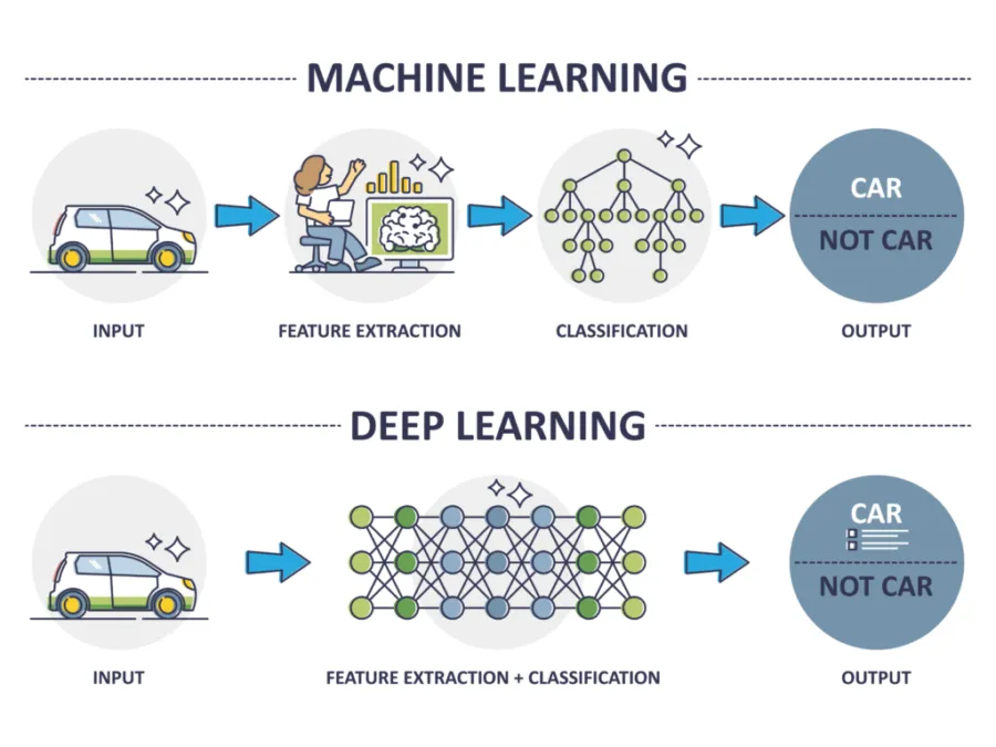
The term "deep learning" can be separated into "deep" and "learning." Learning, in an abstract sense, is the cognitive process of moving from unknown to known by computation, judgment, and reasoning. To enable machines to learn, researchers introduced the concept of artificial neural networks, which mimic biological neurons connected into large networks.

For example, teaching 1+1=2 to a neural network involves repeatedly providing examples until the network learns the mapping. By exposing the network to many examples of arithmetic, it can learn to perform addition. Deep learning extends this idea to more complex tasks such as autonomous driving, speech recognition, machine translation, instant visual translation, and object recognition—for example, mobile voice assistants or face recognition systems in public transit stations.

2.2 Handwritten digit recognition demo

This demo walks through a complete process for recognizing handwritten digits using deep learning. The goal is to train a model on many labeled images so it can predict the digit in unseen images.

Overall approach:

• Train the model on 60,000 labeled images.
• Test the model on 10,000 images the model has not seen during training.
• Repeat training and testing until satisfactory performance is reached.

Program execution steps:

1. Train on 60,000 images.
2. Test on 10,000 images not used in step 1.
3. Repeat steps 1 and 2 as needed.

Understand the function of each module and grasp the overall code flow.

Development environment

Language: Python 3.10.11

IDE: Jupyter Notebook

Framework: TensorFlow 2.4.1

1. Prepare data

import tensorflow as tf from tensorflow.keras import datasets, layers, models # Load dataset (train_images, train_labels), (test_images, test_labels) = datasets.mnist.load_data() # Output data shapes train_images.shape, test_images.shape

((60000, 28, 28), (10000, 28, 28))

Prepare 60,000 labeled training images and 10,000 test images. The shape (60000, 28, 28) indicates 60,000 images of 28x28 pixels.

Visualization

Use matplotlib to display sample images from the dataset.

import matplotlib.pyplot as plt # Set figure size to 20x12 inches plt.figure(figsize=(20,12)) for i in range(20): # Arrange subplots as 5 rows and 10 columns, i+1 selects the subplot plt.subplot(5,10,i+1) # Remove axis ticks plt.xticks([]) plt.yticks([]) # Show image plt.imshow(train_images[i], cmap=plt.cm.binary) # Show label plt.xlabel(train_labels[i]) plt.show()

Adjust image format

Reshape images to the required format for model input.

# Adjust data to the required formattrain_images = train_images.reshape((60000, 28, 28, 1))test_images = test_images.reshape((10000, 28, 28, 1))# 输出数据sahpetrain_images.shape,test_images.shape,train_labels.shape,test_labels.shape

((60000, 28, 28, 1), (10000, 28, 28, 1), (60000,), (10000,))

The shape (60000, 28, 28, 1) denotes 60,000 grayscale images of size 28x28; the final 1 indicates a single channel (grayscale). A value of 3 would indicate RGB images.

2. Build the neural network model

Input images are digitized, then convolutional layers extract features, and fully connected layers classify the digit based on those features. A typical structure includes input, convolutional, flatten, fully connected, and output layers.

• Input layer: feeds data into the network.
• Convolutional layer: uses kernels to extract image features.
• Flatten layer: flattens multidimensional data to one dimension, typically between conv and dense layers.
• Fully connected layer: further processes extracted features.
• Output layer: produces final predictions.

Both convolutional and fully connected layers extract features but use different mechanisms.

model = models.Sequential([ # layers.Conv2D(32, (3, 3), input_shape=(28, 28, 1)), # Convolutional layer: extract image features layers.Flatten(), # Flatten layer: compress 2D image into 1D layers.Dense(100), # Fully connected layer: further compress features layers.Dense(10) # Output layer: produce results]) #?Print network structure

3. Compile the model

Set the optimizer, loss function, and evaluation metric. The optimizer helps training; the loss function measures prediction error; the metric evaluates model performance.

model.compile(optimizer='adam', # adam is a type of optimizer loss=tf.keras.losses.SparseCategoricalCrossentropy(from_logits=True), # a method for computing the loss function ??????????????metrics=['accuracy'])??# Use accuracy to evaluate the model

4. Train the model

Train with training data and validate with test data. epochs specifies the number of training iterations.

5. Prediction

# Display the image we want to predict plt.imshow(test_images[1])

Output the prediction array for the first image in the test set.

pre = model.predict(test_images) pre[1]

array([ 12.474585 , 1.1173537, 21.654232 , 16.206923 , -10.989567 , 17.235504 , 19.404213 , -22.553476 , 13.221286 , -10.19972 ], dtype=float32)

The array corresponds to digits 0–9; the index of the largest value is the predicted digit.

import numpy as np # Output prediction pre_num = np.argmax(pre[1]) print("Predicted result:",pre_num)

Predicted result: 2

Summary

This walkthrough used arithmetic and a handwritten digit recognition demo to illustrate what deep learning is and how a typical deep learning program is structured. The demo implemented handwritten digit recognition with TensorFlow 2 and covered the main steps in a complete workflow.